Real-world uncertainty makes decision making hard. Conversely, without uncertainty decisions would be easier. For example, if a cafe knew exactly 10 customers would want a bagel, then they could make exactly 10 bagels in the morning; if a factory’s machine could make each part exactly the same, then quality control to ensure the part’s fit could be eliminated; if a customer’s future ability to pay back a loan was known, then a bank’s decision to underwrite the loan would be quite simple.
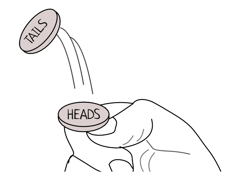
Uncertainty in the outcome of a coin flip can be represented by a probability distribution.
In this chapter, we learn to represent our real-world uncertainty (e.g. demand for bagels, quality of a manufacturing process, or risk of loan default) in mathematical and computational terms. We start by defining the ideal mathematical way of representing uncertainty, namely by assigning a probability distribution to a random variable. Next, we look at modelling real-world uncertainty graphically, mathematically, and in code. Lastly, we learn to describe our uncertainty in a random variable using exact mathematical expressions and their pragmatic computational approximations known as representative samples.
2.1 Random Variables With Assigned Probability Distributions
Think of a random variable as a mapping of outcomes that interest us to probabilities we assign to each potential measurement of those outcomes. For us business folk, we can often think of this mapping as a table with outcomes on the left and probabilities on the right; take this table of coin flip outcomes as an example:
Outcome
Probability
HEADS
50%
TAILS
50%
Table 2.1: Using a table to represent the probability distribution of a coin flip.
While Table 2.1 might be adequate to describe the mapping of coin flip outcomes to probability, as we make more complex models of the real-world, we will want to take advantage of the concise (and often terse) notation that mathematicians would use. In addition, we want to gain fluency in math world notation so that we can successfully traverse the bridge between real world and math world. Random variables are the fundamental math world representation that create the foundation of our studies, so please resist any temptation to not learn the subsequent mathematical notation.
2.1.1 Some Math Notation for Random Variables
Mathematicians love using Greek letters, please do not be intimidated by them - they are just letters. You will learn lots of lowercase letters like (alpha), (beta), (mu), (omega), and (sigma). And also some of their uppercase versions like (omega) as the uppercase of . See the whole list at wikipedia.org.
Above, a random variable was introduced as a mapping of outcomes to probabilities. And, this is how you should think of it most of the time. However, to start gaining fluency in the math-world definition of a random variable, we will also view this mapping process as not just one mapping, but rather a sequence of two mappings: 1) the first mapping is actually the “true” probability-theory definition of a random variable - it maps all possible outcomes to real numbers, and 2) the second mapping, known as a probability distribution in probability theory, maps the numbers from the first mapping to real numbers representing how plausibility is allocated across all possible outcomes - we often think of this allocation as assigning probability to each outcome.
For example, to define a coin flip as a random variable, start by listing the set of possible outcomes (by convention, the greek letter is often used to represent this set and it is called the sample space):
Please note that the full mathematical formalism of random variables is not discussed here. For applied problems, thinking of a random variable as representing a space of possible outcomes governed by a probability distribution is more than sufficient.
The outcomes in a sample space must be 1) exhaustive i.e. include all possible outcomes and 2) mutually exclusive i.e. non-overlapping.
Then pick an an uppercase letter, like , to represent the random variable (i.e. an unobserved sample from ) and explicitly state what it represents using a short description:
where is read “defined as”.
When real-world outcomes are not interpretable real numbers (e.g. heads and tails), define an explicit mapping of these outcomes to real numbers:
For coin flip examples, it is customary to map heads to the number 1 and tails to the number 0. Thus, is a concise way of saying “the coin lands on tails” and likewise means “the coin lands on heads”. The terse math-world representation of a mapping process like this is denoted:
Mathematicians use the symbol to represent the set of all real numbers.
where you interpret it as “random variable maps each possible outcome in sample space omega to a real number.”
The second mapping process then assigns a probability distribution to the random variable. By convention, lowercase letters, e.g. , represent actual observed outcomes. We call the realization of random variable and define the mapping of outcomes to probability for every (read as “in” and interpret it to mean “for each possible realization of random variable ”). As you would already guess, we have 100% confidence that one of the outcomes will be realized (e.g. heads or tails), so as such and by convention, we allocate 100% plausibility (or probability) among the possible outcomes. In this book, we will use , to denote a function that maps each possible realization of a random variable to its corresponding plausibilty measure and use a subscript to disambiguate which random variable is being referred to when necessary. For the coin flip example, we can use our newly learned mapping notation to demonstrate this:
There are several conventions for representing this mapping function which takes a potential realization as input and provides a plausibility measure as output. This textbook uses all of them. Right now, you see or more simply just , but other equally valid notation will use , , or . Knowing that there is not just one standard convention will prove useful as you read other texts about probability. After a while, this change of notation becomes less frustrating.
where you interpret it as “probability density function maps each possible realization of to a number from 0 to 1.” is notation for a number on the interval from 0 to 1; the square brackets mean the interval is closed and hence, the mapping of an outcome to exactly 0 or 1 is possible. For a coin flip, maps to for all plausible values of as shown in Table 2.2. Try not to get lost in the notation by realizing a simple table is able to capture this double-mapping process of 1) outcome to real number, and 2) real number to plausibility measure:
Outcome
Realization ()
HEADS
1
0.5
TAILS
0
0.5
Table 2.2: Probability distribution for random variable represented as a table showing how real-world outcomes are mapped to real numbers and how 100% plausibility is allocated between all of the outcomes.
can be interpreted as the plausability assigned to random variable taking on the value . For example, means that or equivalently that the probability of heads is 50%.
To reiterate how a random variable is a sequence of two mapping processes, notice that Table 2.2 has these features:
It defines a mapping from each real-world outcome to a real number.
It allocates plausability (or probability) to each possible realization such that we are 100% certain one of the listed outcomes will occur.
2.2 The Bernoulli Distribution
“[We will] dive deeply into small pools of information in order to explore and experience the operating principles of whatever we are learning. Once we grasp the essence of our subject through focused study of core principles, we can build on nuanced insights and, eventually, see a much bigger picture. The essence of this approach is to study the micro in order to learn what makes the macro tick.” - Josh Waitzkin
While the coin flip example may seem trivial, we can learn a lot from it. As Josh Waitzkin advocates (Waitzkin 2007), we should “learn the macro from the micro.” In other words, master the simple before moving to the complex. Following this guiding principle, we will try to keep things simple. Let’s model uncertain outcomes where there are two possibilities - like a coin flip, but now we assume the assigned probabilities do not have to be 50%/50%. Somewhat surprisingly, this small abstraction now places an enormous amount of real-world outcomes within our math-world modelling capabilities:
Waitzkin, Josh. 2007. The Art of Learning: A Journey in the Pursuit of Excellence. Simon; Schuster.
Figure 2.1: Ars Conjectandl - Jacob Bernoulli’s post-humously published book (1713) including the yet-to-be-named Bernoulli distribution.
Will the user click my ad?
Will the drug lower a patient’s cholesterol?
Will the new store layout increase sales?
Will the well yield oil?
Will the customer pay back their loan?
Will the passenger show up for their flight?
Is this credit card transaction fraudulent?
The Bernoulli distribution, introduced in 1713 (see Figure 2.1), is a probability distribution used for random variables of the following form:
Outcome
Realization ()
Failure
0
Success
1
Table 2.3: Lookup table describing the mapping process where follows a Bernoulli distribution.
where represents the probability of success - notice that the following must hold to avoid non-sensical probability allocations .
In Table 2.3, is called a parameter of the Bernoulli distribution. Given the parameter(s) of any probability distribution, you can say everything there is to know about a random variable following that distribution; this includes the ability to know all possible outcomes as well as their likelihood. For example, if follows a Bernoulli distribution with , then you know that can take the value of 0 or 1, that , and lastly that
2.3 Unifying Narrative, Math, and Code for a Bernoulli RV
With all of this background, we are now equipped to model uncertainty in data that has two outcomes. The way we will represent this uncertainty is using three forms: 1) a graphical model to capture narrative, 2) a statistical model to rigorously define a mathematical representation of the graphical model, and 3) a computational model to represent the math in code so a computer can help us.
2.3.1 Graphical Model of A Bernoulli RV
The graphical model is simply an oval - yes, we will draw random variables as ovals because ovals are not scary, even to people who don’t like math:
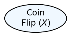
Now, let’s draw an oval using python (Figure 2.2). (TODO: Code to do this discussed in later chapter.)
Figure 2.2: A random variable represented as an oval, a “node”, representing a single unknown coin flip.
Believe it or not, mathematicians and statisticians both love these random-variable ovals; they provide an intuitive way to marry two well-developed mathematical fields, probability theory and graph theory. We will discuss these fields in a later chapter (TODO: add reference). For now, let’s know that Figure 2.2 draws an oval that math-gurus call a node. Our non-technical stakeholders will appreciate us drawing nodes because they are intuitive; they describe some interpretable phenomenon in word. We will appreciate them as a stepping stone towards creating statistical models; the parenthetic text in Figure 2.2, , defines the shorter math notation we will use to refer to this node. The combination of our node drawings and our statistical models form key components of a larger yet-to-be-learned concept known as probabilistic graphical models.
2.3.2 Statistical Model of A Bernoulli RV
For every node used to capture an uncertainty-driven narrative, like a coin flip, a statistical model marries that node to a data-generating process defined using the language of probability. We call this marriage the statistical model and use two key symbols for communication: 1) : a symbol equating concise math notation for a random variable to a real-world description of observed data, and 2) : a symbol to assign a probability distribution to a random variable:
The tilde, , is read “is distributed”; so you say “X is distributed Bernoulli with parameter .”
We will see in future chapters that the graphical model and statistical models are more intimately linked than is shown here, but for now, suffice to say that the graphical model is good for communicating uncertainty to stakeholders more grounded in the real-world and the statistical model is better for communicating with stakeholders in the math-world.
2.3.3 Computational Models of A Bernoulli RV
2.3.3.1 Representative Samples
Despite our ability to represent probability distributions using precise mathematics, uncertainty modelling in the practical world is always an approximation. Does a coin truly land on heads 50% of the time (see [wikipedia article on fair coins] (https://en.wikipedia.org/wiki/Checking_whether_a_coin_is_fair))? Its hard to tell. One might ask, how many times must we flip a coin to be sure? The answer might surprise you; it could take over 1 million tosses to reach an estimate that a coin lies within 0.1% of the observed proportion of heads. That is a lot of tosses. So in the real world, seeking that level of accuracy becomes impractical. Rather, we are seeking a model that is good enough; a model where we believe in its insights and are willing to follow through with its recommendations.
A representative sample is an incomplete collection or subset of data that exhibits a specific type of similarity to a complete collection of data from an entire (possibly infinite) population. For our purposes, the similarity criteria requires that an outcome drawn from either the sample or the population is drawn with similar probability.
Instead of working with probability distributions directly as mathematical objects, we will most often seek a representative sample and treat them as computational objects (i.e. data). For modelling a coin flip, the representative sample might simply be a list of and generated by someone flipping a coin or by a computer simulating someone flipping a coin.
Turning a mathematical object into a representative sample using Python is quite easy as Python (and available packages) can be used to generate random outcomes from a sequence of integers, a supplied array of values, or just about all well-known probability distribution. To generate samples from a random coin flip, we will use this hard-to-say, but easier-to-execute sequence made possible by the numpy package: 1) import the default_rng function from the random module of the numpy package, 2) call default_rng() to get a Generator instance and assign it to a variable using the typical name rng, and 3) use the choice method of the newly created instance to return an array of outcomes:
# import just the default_rng functionfrom numpy.random import default_rngsuccessProb =0.5# probability of "heads" or "success"failProb =1- successProb # prob. of "tails" or "failure"# seed argument so you and I get same randomnessrng = default_rng(seed =111) rng.choice(a = [0,1], size =7, p=[failProb, successProb])
array([0, 0, 1, 1, 1, 0, 1])
The default_rng() function takes an integer seed argument. If your computer and my computer supply the same integer argument to this function (e.g. 111), then we will get the same random numbers even though we are on different computers. I use this argument when I want your “random” results and my “random” results to match exactly.
where the three 0’s and four 1’s are the result of the size=7 coin flips.
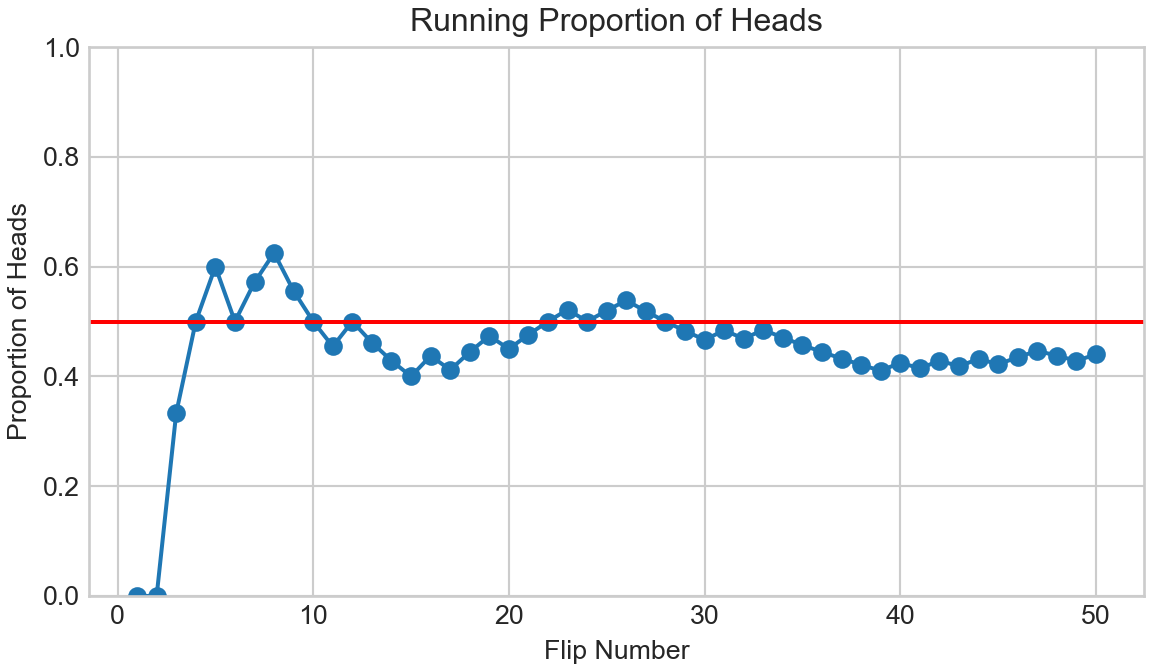
Notice that one might be reluctant to label this a representative sample as the proportion of 1’s is 0.57 and not the 0.5 that a representative sample would be designed to mimic. In fact, we can write code to visualize the proportion of heads as a function of the number of coin flips:
import pandas as pdfrom numpy import cumsum, arange, mean# if on google Colab, need to update matplotlib# !pip install matplotlib --upgradeimport matplotlib.pyplot as pltplt.style.use("seaborn-whitegrid")# reset random number seed so flips will be same as aboverng = default_rng(seed =111) numFlips =50# create pandas dataframe from a dictionary# range(1, numFlips+1) is sequence of 1 to 50df = pd.DataFrame({"flipNum": range(1, numFlips+1), "coinFlip": rng.choice(a = [0,1], size = numFlips, p=[failProb, successProb])})df["headsProportion"] = df.coinFlip.cumsum() / df.flipNum## plot the results using matplotlib object-oriented interfacefig, ax = plt.subplots(figsize=(6, 3.5), layout='constrained')ax.plot("flipNum","headsProportion", data = df)ax.scatter("flipNum","headsProportion", data = df)ax.set_ylim(0,1);ax.axhline(0.5, color ="red")ax.set_xlabel("Flip Number")ax.set_ylabel("Proportion of Heads")ax.set_title("Running Proportion of Heads")plt.show()
Figure 2.3: Even after 50 coin flips, the proportion of heads can remain far from 50%.
Notice that even after 40 coin flips, the sample is far from representative as the proportion of heads is 0.414. Even after 1,000 coin flips (i.e. numFlips = 1000), the proportion of heads, 0.496, is still just an approximation as it is not exactly 0.5.
Well if 1,000 coin flips gets us an approximation close to 0.5, then 10,000 coin flips should get us even closer. To explore this idea, we generate ten simulations of 10,000 coin flips and print out the average proportion of heads for each:
rng = default_rng(seed =111)# use _ in for loop when you do not need to reference# specific values during iteration; a "throwaway" variablefor _ inrange(10): proportionOfHeads = mean(rng.choice(a = [0,1], size =10000, p=[failProb, successProb]))print(proportionOfHeads)
From the above, we can calculate the average distance away from the exact proportion 0.5 is 0.00322. So on average, it appears we are around 0.6% away from the true value. This is the reality of representative samples; they will prove enormously useful, but are still just approximations of the underlying mathematical object - in this case, that has a known 50% long-run average proportion of heads. If this approximation bothers you, remember the mathematical object is just an approximation of the real-world object. Might it be possible that certain coins are weighted in one way or another to deviate - even ever so slightly - from the ideal? Of course, but it does not mean the approximations are useless … on the contrary, we will see how powerful the math-world and computation-world can be in bringing real-world insight.
2.4 Multi-Node Graphical Models
So far, we have represented uncertainty in a simple coin flip - just one random variable. As we try to model more complex aspects of the business world, we will seek to understand relationships between random variables (e.g. price and demand for oil). Starting with our simple building block of drawing an oval to represent one random variable, we will now draw multiple ovals to represent multiple random variables. Let’s look at an example with more than one random variable:
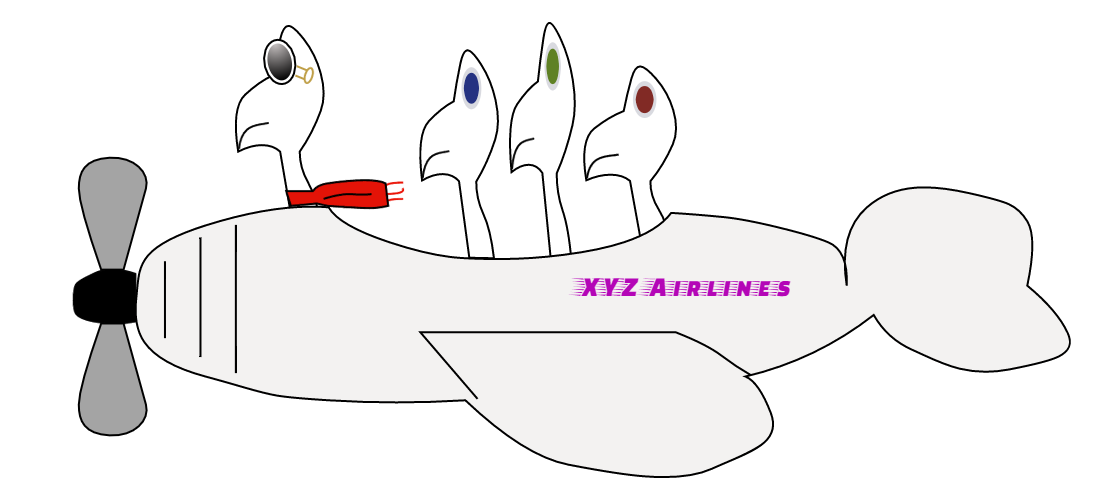
Figure 2.4: How many passengers will show up if XYZ Airlines accepts three reservations?
Example 2.1 The XYZ Airlines company owns the one plane shown in Figure 2.4. XYZ operates a 3-seater airplane to show tourists the Great Barrier Reef in Cairns, Australia. The company uses a reservation system, wherein tourists call in advance and make a reservation for aerial viewing the following day. Unfortunately, often passengers holding a reservation might not show up for their flight. Assume that the probability of each passenger not showing up for a flight is 15% and that each passenger’s arrival probability is independent of the other passengers. Assuming XYZ takes three reservations, use your ability to simulate the Bernoulli distribution to estimate a random variable representing the number of passengers that show up for the flight. How many passengers will show up if XYZ Airlines accepts three reservations?
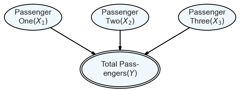
To solve Example 2.1, we take the real-world problem and represent it mathematically with three random variables: 1) whether passenger 1 shows up, 2) whether passenger 2 shows up, and 3) whether passenger 3 shows up. And to answer the question of how many passengers show up, we define one more random variable, . Since is a function of the other three random variables, we will use arrows in our graphical model to indicate this relationship:
Figure 2.5: A multi-node graphical model. Edge direction indicates influence flowing from the parent node to the child node. Nodes with double perimeters are deterministic functions of their parent nodes.
For each node in Figure 2.5, we explicitly define both a real-world description and a probability distribution. Using details from the narrative in Example 2.1 and our graphical depiction in Figure 2.5, we can state our statistical model:
We will use the terms generate samples and simulate interchangeably. Both refer to the process mathematicians refer to as Monte Carlo sampling. For us, we use sampling to repeatedly generated random variables that are combined according to a graphical model recipe, and are designed to mimic the uncertainty of some real-world phenomenon.
The above gives us a recipe to generate a representative sample of the number of passengers who show up for the flight; we simulate three Bernoulli trials and add up the result. Computationally, we can create a data frame to simulate as many flights as we want. Let’s simulate 1,000 flights and see the probabilities associated with :
# place parameters that might change at top of script for conveniencenumFlights =1000probShow =0.85probNoShow =1- probShowrng = default_rng(seed =111) # create data frame to store simulated flightsflightDF = pd.DataFrame({"simNum": range(1, numFlights+1),"pass1": rng.choice(a = [0,1], size = numFlights, p=[probNoShow, probShow]),"pass2": rng.choice(a = [0,1], size = numFlights, p=[probNoShow, probShow]),"pass3": rng.choice(a = [0,1], size = numFlights, p=[probNoShow, probShow])})# get total passengers for each flightflightDF["totalPass"] = flightDF.pass1 + flightDF.pass2 + flightDF.pass3# view first few 5 rows of flightDFflightDF.iloc[:5,:]
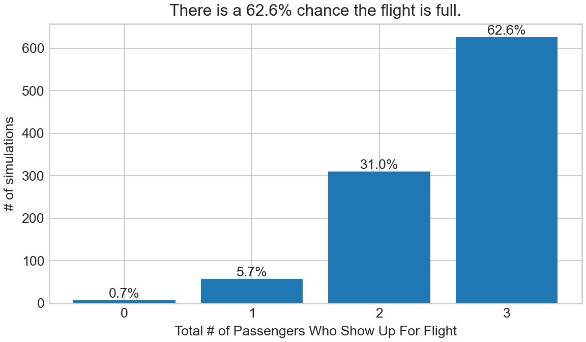
The first five of these simulations, shown above, generated three flights with three passengers showing up and two flights with two passengers showing up. Five simulated flights definitely does not give us a representative sample, but our ability to simulate 1,000 flights just might give us more faith in our simulation. Figure 2.6 summarizes our complete simulation to answer the motivating question, “how many passengers will show up if XYZ Airlines accepts three reservations?”
## plot the results using matplotlib object-oriented interfacefrom numpy import uniquefig, ax = plt.subplots(figsize=(6, 3.5), layout='constrained')# np.unique returns tuple that we unpack into unique values and their counts values, counts = unique(flightDF.totalPass, return_counts=True)pctOfCount = (counts /sum(counts) *100).round(1)pctLabels = [str(pctNum)+"%"for pctNum in pctOfCount]barReference = ax.bar(values, counts)ax.bar_label(barReference, labels = pctLabels);ax.set_xticks(values);ax.set_xlabel('Total # of Passengers Who Show Up For Flight');ax.set_ylabel('# of simulations');ax.set_title('There is a '+ pctLabels[-1] +' chance the flight is full.');plt.show()
Figure 2.6: Our visual response to “how many passengers will show up?”
So, assuming we created a representative sample, Figure 2.6 provides nicely presented probability estimates for a random variable, , whose distribution was not Bernoulli. Rather, is constructed as the sum of three Bernoulli random variables. Combining random variables using graphical models will prove tremendously powerful as the complexity of our narratives grow.
You may be wondering how much the approximated probabilities for the number of passengers might vary with a different simulation. The best way to find out is to try it again. Remember to eliminate or change the seed argument prior to trying the simulation again, otherwise you will get the same results.
Success in using simulation to create the revealing graph of Figure 2.6 is the result of carefully transitioning from narrative to math, and from math to code - a theme we will see recurring throughout this text. Note, the graph above is just our response to one question, but with representative sample in hand, we can now answer all sorts of question; questions like “what is the probability there is at least one empty seat?” This is the same as saying what is or equivalently . And the answer, albeit an approximate answer, is 37.4%.
2.5 Mathematics As A Simulation Shortcut
Simulation will always be your friend in the sense that if given enough time, a simulation will always give you results that approximate mathematical exactness. The only problem with this friend is it is sometimes slow to yield representative results. In these cases, sometimes mathematics provides a shortcut. The shortcut we study here is to introduce a new probability distribution that mimics the real-world phenomenon we are interested in and that mathematicians have exact analytical results we can leverage for answering probabilistic queries instantaneously (as opposed to waiting for 1,000 or more simulations).
2.5.1 Probability Distributions and Their Parameters
Named probability distributions are cool math shortcuts we can use to avoid simulation. Each named distribution (e.g. Bernoulli, normal, uniform, etc.) has a set of parameters (i.e. values provided by you) that once specified tell you everything there is to know about a random variable - let’s call it . Previously, we learned that is the one parameter of a Bernoulli distribution and it can be used to describe as such:
Once we give a value, say , then we know everything there is to know about random variable . Specifically, we know its possible values (i.e. 0 or 1) and we know the probability of those values:
Realization ()
0
1
This is the shortcut. Once you name a distribution and supply its parameters, then its potential values and their likelihood are fully specified.
2.5.2 The Binomial Distribution
The two parameters of a binomial distribution map to the real-world in a fairly intuitive manner. The first parameter, , is simply the number of Bernoulli trials your random variable will model. The second parameter, , is the probability of observing success on each trial. So if and , then an outcome of means that four heads were observed in 10 coin flips.
A particularly useful two-parameter distribution was derived as a generalization of a Bernoulli distribution. None other than Jacob Bernoulli himself realized that just one Bernoulli trial is sort of uninteresting (would you predict the next president by polling just one person?). Hence, he created the binomial distribution.
The binomial distribution is a two-parameter distribution. You specify the values for the two parameters and then, you know everything there is to know about a random variable which is binomially distributed. The distribution models scenarios where we are interested in the cumulative outcome of successive Bernoulli trials - something like the number of heads in multiple coin flips or the number of passengers that arrive given three reservations. More formally, a binomially distributed random variable, let’s call it , represents the number of successes in Bernoulli trials where each trial has success probability . Thus, and are the two-parameters that need to be specified for a Binomial-distributed random variable.
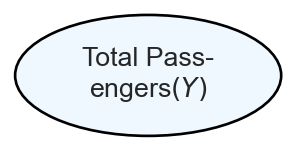
Going back to our airplane in Example 2.1, we can take advantage of the mathematical shortcut provided by the binomial distribution and use the following graphical/statistical model combination to yield exact results. The graphical model is just a simple oval:
Figure 2.7: The graphical model of number of passengers who show up for the XYZ airlines tour.
And, our mathematical shortcut is to specify a single binomial random variable; avoiding the simulation and summing of three simulated Bernoulli random variables. The statistical model is represented like this:
2.5.3 Exact Answers Versus Sample-Based Approximations
Figure 2.6 represents our simulated total number of passengers arriving at a flight; we found that approximately 62.6% of flights would be full. To get this number, samples were generated using the numpy.random module. Typically, this workflow of sample generation and its subsequent inspection is how we will model and answer probabilistic queries about real-world phenomenon; phenomenon that are too complex for mathematics to have clean answers. However, when exact mathematical expressions are available, we save computation time and reduce approximation error by using them.
For just about any named probability distribution, like the binomial distribution, exact expressions exist; we find them in Python’s scipy.stats module. We just need to know the right functions/methods to use. Thanks to an established convention, any random variable created using scipy.stats will have methods to extract exact answers for probabilistic queries. The most useful methods are shown for a generic scipy.stats random variable named foo:
foo is called a placeholder name in computer programming. The word foo itself is meaningless, but you will substitute more meaningful words in its place. In the examples here, foo is a stand-in for a defined random variable, e.g. foo = stats.binom(n, p) or foo = stats.norm(mean,sd).
foo.pmf() - is the probability mass function(PMF). Only used for discrete random variables, the PMF answers “what is the probability random variable (”big X”) is observed to be equal to a specified (“little x”), i.e. ?” A user inputs and the parameters of ’s distribution, the function returns . Typical math notation for this function is , , or . Python uses the letter as the argument to this method; equivalent to our .
foo.pdf() - is the probability density function. Only used for continuous random variables, this number is not interpretable as a probability and does not directly help to answer any probabilistic queries (see this Khan Academy video for more background information). Typical math notation for this function is , called “little f”.
foo.cdf() - is the cumulative distribution function (CDF) and has the same interpretation for both discrete and continuous random variables. The CDF answers “what is the probability random variable (”big X”) is observed to be equal to or less than some value (“little x”), i.e. ?” User inputs argument (continuous) or analogously (discrete), the CDF returns a probability such that (or ). Typical math notation for this function is , called “big F”.
foo.ppf() - is the percent point function or quantile function. It is known as the inverse of the CDF function. User inputs argument , a probability, and the method returns the value such that . Corresponding math notation for this function is , “the inverse CDF”.
Using the statistical model of Equation 2.1 and our newly learned functions from scipy.stats, we can now exactly answer our question of “How many passengers will show up if XYZ Airlines accepts three reservations?” Here is how to find the probability that the flight is full, :
import scipy.stats as stats# codify statistical model of @eq-binomn, p =3, 0.85#python trick used here called unpacking a tuplenumPassRV = stats.binom(n, p)# the probability of exactly 3 passengersnumPassRV.pmf(3)
0.6141249999999999
Note that our approximation from Figure 2.6 of 62.6% is good, but not perfect, the exact result above gives us 61.4%. By the law of large numbers, our approximation would get infinitely better with larger and larger numbers of simulated draws.
When doing exact inference, clever use of the CDF function is usually needed to answer probabilistic queries. For example, to answer “what is the probability the plane has more than one passenger?”, we seek . From knowing that must take on some value, we have:
which can be rearranged:
and then solved computationally:
# the probability of more than 1 passenger1- numPassRV.cdf(1)
0.93925
Again, this exact answer is very close, but not identical, to our previously approximated answer of 93.6%.
Exact answers are both simpler and faster than the approximation code run earlier. Hence, when we can take mathematical shortcuts, we will to save time and reduce the uncertainty in our results introduced by approximation error. That being said, more complex models of the real-world and later chapters of this book will not have exact answers; approximation methods will be the focus of our efforts.
2.6 Joint Distributions Tell You Everything
2.6.1 Joint Distributions
Do not let the fancy calligraphy notation of scare you - its equivalent to last chapter’s . A frustration of learning math is varying conventions are employed to name things. The fancy is just a function that takes input and outputs a probability. In this textbook and others, you will see all sorts of equivalent notation for a probability function including where is replaced by a set of random variable values. The function input, , represents random variables; supply realizations to the function and the function returns a probability of seeing that realization.
The most complete method of reasoning about sets of random variables is by having a joint probability distribution. A joint probability distribution, , assigns a probability value to all possible assignments or realizations of sets of random variables. My goal here is to 1) introduce you to the notation of joint probability distributions and 2) to convince you that if you are given a joint probability distribution that you would be able to answer some very useful questions related to probability.
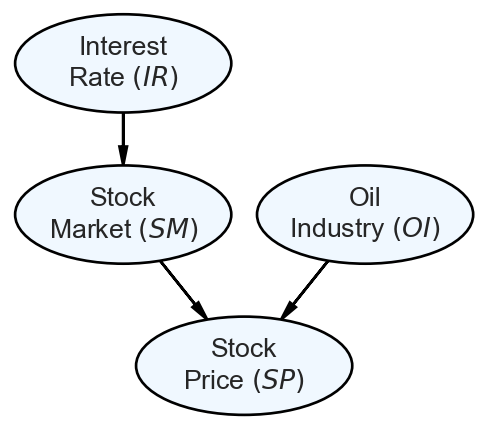
Consider the graphical model from Shenoy and Shenoy (2000) and depicted in Figure Figure 2.8.
Shenoy, Catherine, and Prakash P Shenoy. 2000. Bayesian Network Models of Portfolio Risk and Return. The MIT Press.
Figure 2.8: Model of how stock prices for oil companies are influenced by other factors.
In Figure 2.8, there are four random variables: 1) Interest Rate, 2) Stock Market, 3) Oil Industry, and 4) Stock Price (assume for an oil company). The arrows between the random variables tell a story of precedence and causal direction: interest rate influences the stock market which then, in combination with the state of the oil industry will determine the stock price (we will learn more about these arrows in the Graphical Models chapter). For simplicity and to gain intuition about joint distributions, assume that each of these four random variables is binary-valued, meaning they can each take two possible assignments:
Random Variable
Set of Possible Values (i.e. )
Note that probability notation on the Internet or in books does not conform to just one convention. I will mix conventions in this book, not to confuse you, but to give you exposure to other conventions you might encounter when going forward on your learning journey outside of this text. Everytime I introduce a slightly changed notation, I will add comments in the margin introducing it.
Thus, our probability space has values corresponding to the possible assignments to these four variables. So, a joint distribution must be able to assign probability to these 16 combinations. Here is one possible joint distribution:
0.016
0.168
0.04
0.045
0.018
0.189
0.012
0.0135
0.004
0.042
0.04
0.045
0.012
0.126
0.108
0.1215
Table 2.4: A joint distribution shown in table form.
Notation note: . Each defines a function where you supply realizations and and the probability function will return . For example, let outcome of a dice roll and outcome of a coin flip. Hence, you can supply potential outcomes, like which means and the function output would be (if you were to do the math).
Collectively, the above 16 probabilities represent the joint distribution - meaning, you plug in values for all four random variables and it gives you a probability. For example, yields a probability assignment of 12.15%.
2.6.2 Marginal Distributions
If its been a while since you have seen the summation notation, , or set notation like , you can do a quick review of them at wikipedia: wikipedia summation entry and wikipedia set entry, respectively.
More generally speaking, a marginal distribution is a compression of information where only information regarding the marginal variables is maintained. Take a set of random variables, (e.g. ), and a subset of those variables (e.g. ). And using standard mathematical convention, let be the set of random variables in that are not in (i.e. . Assuming discrete random variables, then the marginal distribution is calculated from the joint distribution . Effectively, when the joint probability distribution is in tabular form, one just sums up the probabilities in each row where .
One might also be curious about probability assignments for just a subset of the random variables. This smaller subset of variables can be called marginal variables and their probability distribution is called a marginal distribution. For example, the marginal distribution for oil industry is notated as and represents a probability distribution over just one of the four variables - ignoring the others. The marginal distribution can be derived from the joint distribution using the formula:
Think of a marginal distribution as a function of the marginal variables. Given realizations of the marginal variables, the function returns a probability. Applying the above formula to determine the marginal distribution of yields a tabular representation of the marginal distribution (Table 2.5).
Realization ()
0.016 + 0.168 + 0.04 +
0.045 + 0.004 + 0.042 +
0.04 + 0.045 = 0.4
0.018 + 0.189 + 0.012 +
0.0135 + 0.012 + 0.126 +
0.108 + 0.1215 = 0.6
Table 2.5: A marginal distribution shown in table form.
2.6.3 Conditional Distributions
If you need a refresher on conditional probability, see the wikipedia article here: https://en.wikipedia.org/wiki/Conditional_probability and the khan academy video here: https://youtu.be/6xPkG2pA-TU.
Conditional distributions can be used to model scenarios where a subset of the random variables are known (e.g. data) and the remaining subset is of interest (e.g. model parameters). For example, we might be interested in getting the conditional distribution of Stock Price () given that we know the Interest Rate. The notation for this is and can be calculated using the definition of conditional probablity:
Think of a conditional distribution as a function of the variables to the left of the conditioning pipe ($ | $) - since they are assumed given, you already know the value for the right-side variables with 100% certainty. You supply realizations of the left-side variables, the function returns a probability.
For our specific problem:
To calculate conditional probabilities when already given the joint distribution, use a two-step process:
To get the marginal distribution, just aggregate the rows in the joint distribution as done in the previous section on marginal distributions.
First, to simplify the problem, calculate the numerator, i.e. the marginal distribution for , and rid ourselves of the variables that we are not interested in:
0.086
0.4155
0.164
0.3345
Then, calculate any conditional distribution of interest by plugging in the given value for and all of the possible values. For example means we need to be able to find a probability for the two outcomes given that we know . Hence, we calculate and :
and,
which yields the following tabular representation of the conditional distribution for :
2.6.4 MAP Estimates
Sometimes, we are not interested in a complete probability distribution, but rather seek a high-probability assignment to some subset of variables. For this, we can use a query (maximum a posteriori query). A finds the most likely assignment of all non-evidentiary variables (i.e. unknown values). Basically, you search the joint distribution for the largest probability value. For example, the maximum a posterior estimate of stock price given would be given by the following formula:
which in natural language asks for the argument (i.e. the realization of stock price) that maximizes the conditional probability . From above, we realize that and and hence, the MAP estimate is that because .
2.6.5 Limitations of Joint Distributions
Why don’t we just use joint probability distributions all the time?” Despite the expressive power of having a joint probability distribution, they are not that easy to directly construct due to the curse of dimensionality. As the number of random variables being considered in a dataset grows, the number of potential probability assignments grows too. Even in the era of big data, this curse of dimensionality still exists.
Generally speaking, an exponential increase is required in the size of the dataset as each new descriptive feature is added.
Let’s assume we have random variables with each having values. Thus, the joint distribution requires probabilites. Even if and , this leads to 17,179,869,184 possibilities (over 17 billion). To make this concrete, a typical car purchase decision might easily look at 34 different variables (e.g. make, model, color, style, financing, etc.). So, to model this decision would require a very large joint distribution which actually dwarfs the amount of data that is available. As a point of comparison, well under 100 million motor vehicles were sold worldwide in 2019 - i.e. less than one data point per possible combination of features. Despite this “curse”, we will learn to get around it with more compact representations of joint distributions. These representations will require less data, but will still yield the power to answer queries of interest; just as if we had access to the full joint distribution.
2.7 Big Picture Takeaways
This chapter is our first foray into representing uncertainty. Our representation of uncertainty takes place in three worlds: 1) the real-world - we use graphical models (i.e. ovals) to convey the story of uncertainty, 2) the math-world - we use statistical models to rigorously define how random outcomes are generated, and 3) the computation-world - we use scipy.stats methods to answer questions about exact distributions and representative samples to answer questions when the exact distribution is unobtainable. As we navigate this course, we will traverse across all these worlds and become experts in unifying narrative, math, and code.
2.8 Getting Help
Google and YouTube are great resources to supplement, reinforce, or further explore topics covered in this book. For the mathematical notation and conventions regarding random variables, I highly recommend listening to Sal Khan, founder of Khan Academy, for a more thorough introduction/review of these concepts. Sal’s videos can be found at https://www.khanacademy.org/math/statistics-probability/random-variables-stats-library.
2.9 Questions to Learn From
Exercise 2.1 Most professional soccer games can end in a tie. If you were to model an individual team’s results for a completed game, how many outcomes would be in the sample space? Enter your answer as an integer.
Exercise 2.2 Most professional soccer games can end in a tie. Assume a team’s outcome, , is defined as follows:
I made the following code to simulate a team’s season (38 games) assuming a 35% chance of winning and a 25% chance of tying:
# import just the default_rng functionfrom numpy.random import default_rnglossProb =0.25## probability of losstieProb =0.4## probability tiewinProb =1- lossProb - tieProb ## probability of win## DO NOT CHANGE THIS LINE - seed used so you and I get same randomnessrng = default_rng(seed =111)outcomeArray = rng.choice(a = [-1,0,1], size =38, p=[tieProb, winProb])## report the sum of the above numpy.ndarray## this represents how many more wins than losses the team has experienced## for the simulated thirty eight game seasonoutcomeArray.sum()
The above code was working just a moment ago and I had a simulated result, but I think I hit DELETE and lost something. Can you please debug the above code? This documentation might help: numpy help documentation
After fixing (not redoing) the code, what value do you get for WINS - LOSSES (i.e outcomeArray.sum())? [Enter answer as an integer]
Exercise 2.3 Let . Assuming , what is the probability that a coin flip lands on tails?
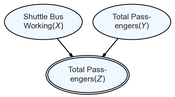
Exercise 2.4 The XYZ Airlines company owns the one plane shown in Figure 2.9. XYZ operates a 3-seater airplane where tourists make a reservation for an aerial excursion with XYZ. Unfortunately, there are two issues. First, the tourists get to the airport via a shuttle bus that is unreliable; when the shuttle bus breaks down or the driver is sick, zero passengers arrive for the flight; this happens about 10% of the time. Second, even if the shuttle bus is operational, passengers holding a reservation might not show up to get on the bus. The probability of each passenger showing up to the bus is 80%; each passenger’s arrival probability is independent of the other passengers. Assuming XYZ takes three reservations, use a Bernoulli random variable () to simulate the shuttle bus working, and a binomial random variable to represent the number of passengers that show up to catch the bus to the plane (). Thus, will represent the number of passengers who make it to the plane as shown below.
Figure 2.9: How many passengers will show up if XYZ Airlines accepts three reservations?
Figure 2.10: The graphical model of number of passengers who show up for the XYZ airlines tour.
Using 4,000 simulated draws of , create an updated plot of Figure 2.6 that shows the new estimates for total passengers who can take the flight. Submit your code by naming the file with your last name as a python script lastName.py or notebook lastName.ipynb.
Exercise 2.5 In this exercise, we explore the concept of a random generator, e.g. rng = default_rng(). Running this code,
from numpy.random import default_rngrng = default_rng()type(rng)
<class 'numpy.random._generator.Generator'>
you discover that the object rng is an instance of the numpy.random._generator.Generatorclass. Google thisnumpy.random._generator.Generator` to get to the generator documentation located at:
Read through this documentation. Take special note of the capital “G” in class numpy.random.Generator, capitalization in Python is a convention used to indicate a class. Also, at the top of the documentation, take note that you construct an instance of that class using numpy.random.default_rng(). To signal your understanding of the documentation, generate a new instance of the Generator class (using the recommended constructor) with the seed value of 111. Immediately after creating the generator, use it with the integers method to simulate 20 random integers, where each with equal probability of all ten values. To prove you understood this, report the sum of those simulated integers here. (Hint: carefully note use of inclusive and exclusive in the documentation)
Exercise 2.6 After defining your statistical model for this question, use scipy.stats to get an exact answer. A shop receives a batch of 1,000 cheap lamps. The odds that a lamp are defective are 0.4%. Let X be the number of defective lamps in the batch. What is the probability the batch contains exactly 2 defective lamps? Enter as decimal with three significant digits.
Exercise 2.7 After defining your statistical model for this question, use scipy.stats to get an exact answer. A shop receives a batch of 1,000 cheap lamps. The odds that a lamp are defective are 0.2%. Let X be the number of defective lamps in the batch. What is the probability the batch contains less than or equal to 2 defective lamps (i.e. P(X≤2))? Enter as decimal with three significant digits.
Exercise 2.8 Suppose we are only interested in the Oil Company Stock Price (). Given the probabilities in the joint distribution of Table 2.4, what is the marginal distribution for (i.e. and )?
Exercise 2.9 Suppose we are interested in both the Stock Market () and the Oil Industry (). We can find the marginal distribution for these two variables, . This is sometimes called a joint marginal distribution; joint referring to the presence of multiple variables and marginal referring to the notion that this is a subset of the original joint distribution. So, given the probabilities in the joint distribution of Table 2.4, what is the marginal distribution for - i.e. give a probability function for
,
,
, and
)?
which are the four possible realizations.
Exercise 2.10 Starting with the joint distribution of Table 2.4, suppose that we learn is low. What is the conditional distribution for (i.e. and )?
Exercise 2.11 Based on the joint distribution in Table 2.4 and letting , what is , the most likely joint assignment?
Exercise 2.12 Continuing from Exercise 3.10, suppose we learn that is low. Let , what is , the most likely joint assignment?
Exercise 2.13 This question will have you combine the concepts of representative samples and joint distributions over sets of random variables. Imagine we are given the below representative sample where each row represents an observation of three potentially correlated random variables, , , :
A
B
C
10
20
30
10
20
30
20
20
30
20
20
30
30
20
30
30
20
10
40
20
10
40
20
10
50
20
10
50
20
10
Using the above as a representative sample, estimate . Enter your probability as a decimal with three significant digits, e.g. 0.125, 0.246, etc.. (disclaimer: 10 samples is usually not enough to be a representative sample, but let’s assume it is for the purposes of this question)