11 Bayesian Linear Models

BuildIt Inc. flips houses - they buy houses to quickly renovate and then sell. Their specialty is building additions on to existing houses in established neighborhoods and then selling the home at prices above their total investment. BuildIt’s decision to move into a neighborhood is based on how sales price fluctuates with square footage. If sales price seems to increase by more than $120 per additional square foot, then they consider that neighborhood to be a good candidate for buying houses. BuildIt is eyeing a new neighborhood and records the square footage and prices of some recent sales transactions.
The following code creates a dataframe with BuildIt’s findings (note: salesPrice is in thousands of dollars):
## make two data arrays representing observations
## of six home sales
salesPrice = [160, 220, 190, 250, 290, 240]
sqFootage = [960, 1285, 1350, 1600, 1850, 1900]
Visually, we can confirm what appears to be a linear relationship between square footage and sales prices by creating a scatterplot with a linear regression line drawn in blue (the experimental seaborn.objects interface within the seaborn package can do this quickly and it is a superior interface, allowing for method chaining, than the standard seaborn interface):
https://seaborn.pydata.org/tutorial/objects_interface.html#
import seaborn as sns
import seaborn.objects as so
import matplotlib.pyplot as plt
from matplotlib import style

(
    so.Plot(x=sqFootage, y=salesPrice)
    .add(so.Dots(pointsize = 12)) ## big points
    .add(so.Line(), so.PolyFit(order = 1)) ## adds regression line
    .label(x="Square Footage", y="Sales Price in (000's)")
    .theme({**style.library["seaborn-whitegrid"]})
    .show()
)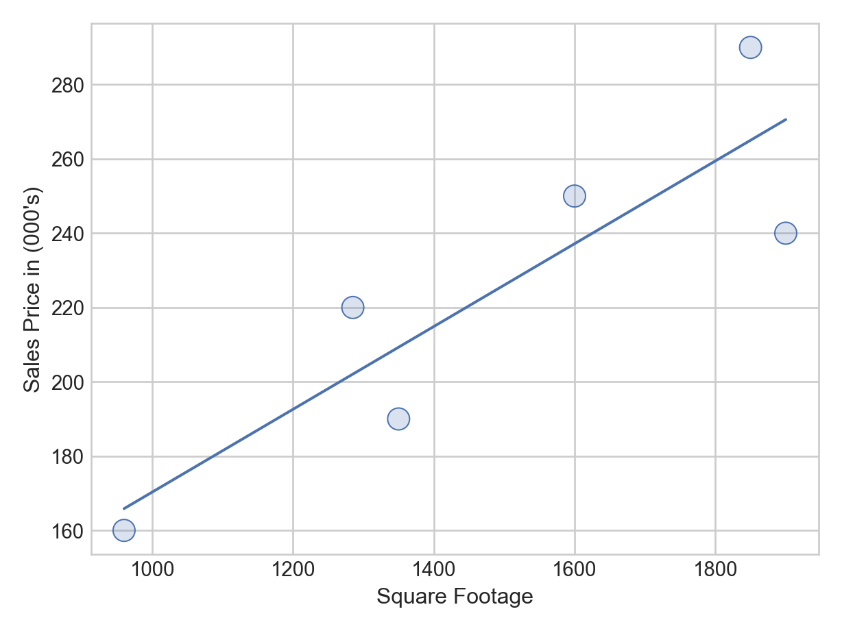
BuildIt is interested in the slope of this line which gives the estimated change in mean sales price for each unit change in square footage. For BuildIt, they want to know if this slope is above $120 per square foot because at that price point the firm is confident it can make money?
Letting,
the linear regression output can be extracted using the numpy.polyfit() function. We will not worry about the coding details here as this is not the type of regression we will use going forward. For now, the first element of the returned array is
import numpy as np
np.polyfit(x = sqFootage, y = salesPrice, deg = 1)
array([ 0.1114099, 58.9064047])Based on the output, the following linear equation is the so-called “best” line:
The model suggests, assuming its assumptions are justified, that BuildIt can anticipate being able to sell additional square footage for about $111 per square foot (i.e. 6 data points, there is obviously going to be tremendous uncertainty in this estimate. A Bayesian model, like we will use below, helps to capture this uncertainty.
11.1 A Simple Bayesian Linear Model
From previous coursework, you are probably familiar with simple linear regression in a non-Bayesian context. Extending this model to our Bayesian context, we will create an observational model with the assumption that our observed data is normally distributed around some line. Let’s use the following notation to describe the line:
where,
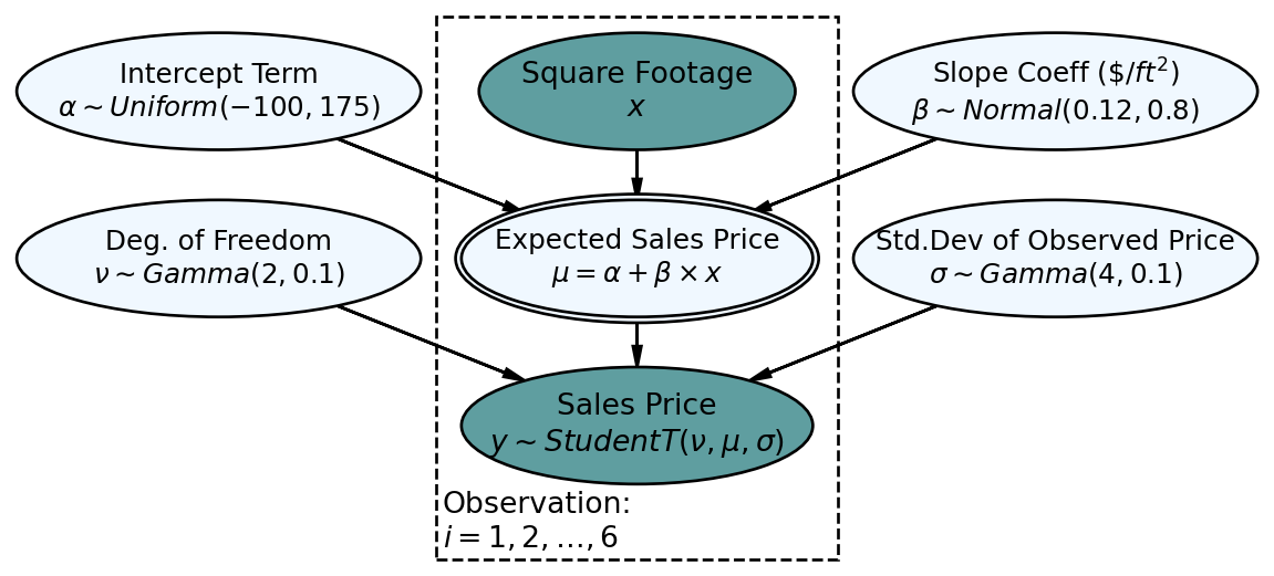
Using a generative DAG, Figure 11.3 presents the Bayesian version of simple linear regression.
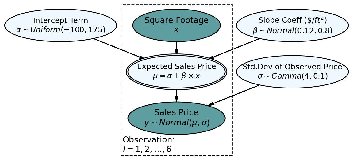
The statistical model of the generative DAG in Figure 11.3 has reasonable priors that we will analyze later - for now, let’s digest the implied narrative. Starting at the bottom:
- Sales Price Node(
- Expected Sales Price Node(
- Square Footage Node(
- All other yet-to-be discussed nodes are outside the Observations plate. Therefore, each posterior draw from the model will contain just one value. The node we are most interested in is Slope Coeff,
A main deficiency of non-Bayesian linear regression lines is that they do not measure uncertainty in slope coefficients very well. Ultimately, we would rather make decisions that do not fall victim to the hubris of a single estimate and instead make informed decisions with measured uncertainty. For us, we seek to investigate all plausible parameter values for the square footage coefficient, not just one.
To highlight the idea of having multiple plausible lines, consider capturing the relationship between sales price and square footage using one of the 6 alternative lines shown using dashed lines in Figure 11.4:
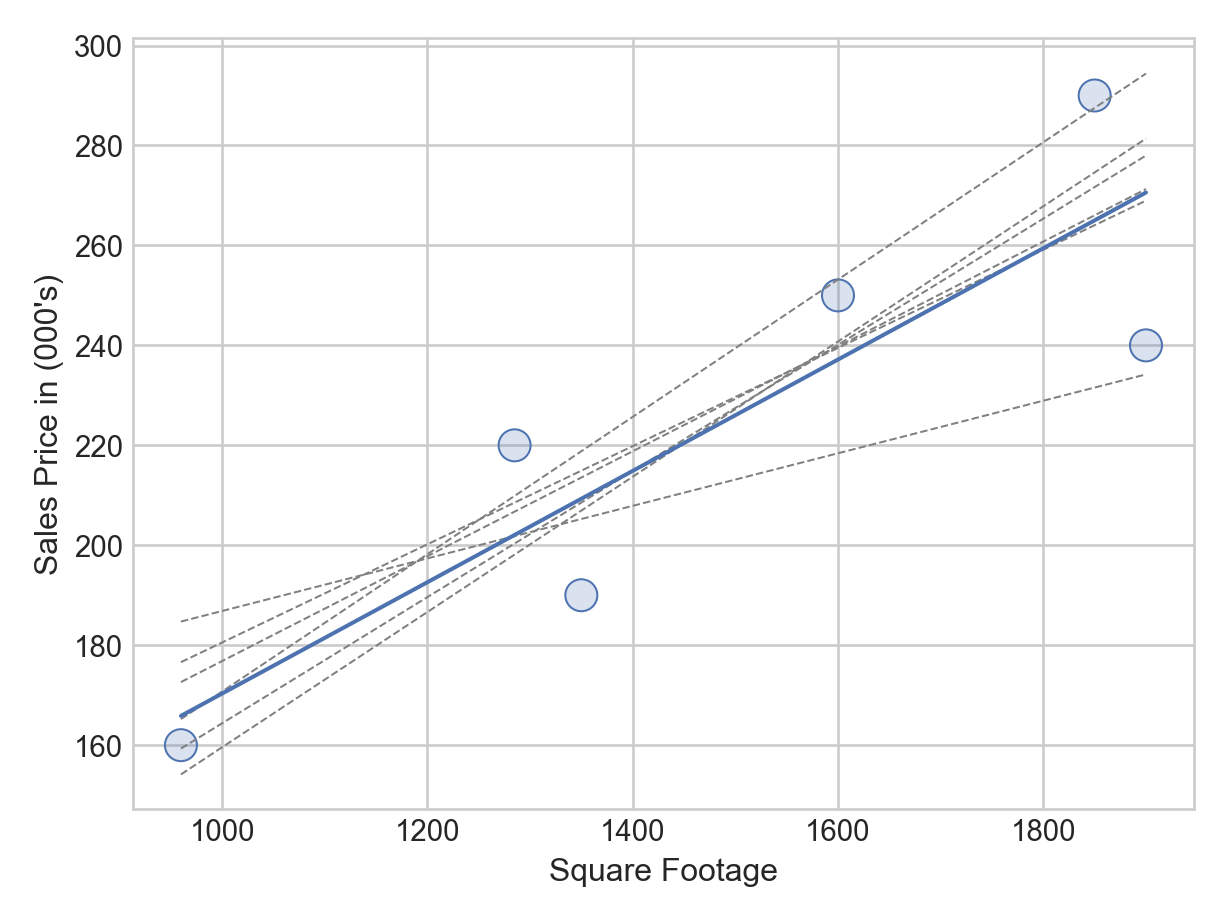
Might the alternative dashed lines of Figure 11.4 also describe the relationship between square footage and the expected sales price of a house? Actually, they do seem reasonable - by golly, there should be multiple plausible lines. So instead of just defining one plausible line, let’s use Bayesian inference to get a posterior distribution over all plausible lines consistent with our model.
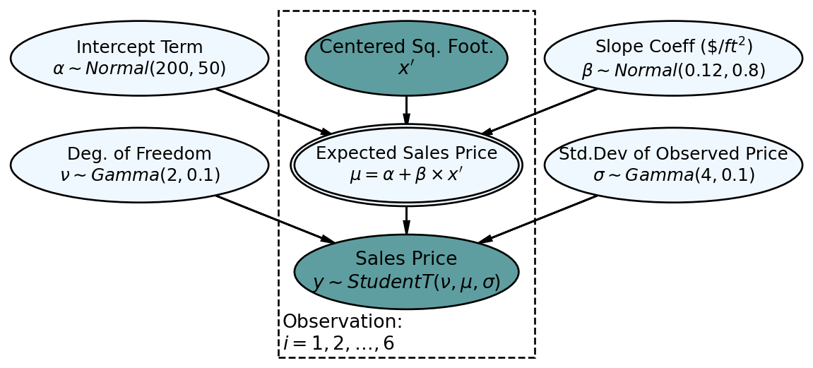
Our interest is in the slope of the plausible lines. Because different slope terms can dramatically affect where the line crosses the y-axis, the intercept term should be allowed to fluctuate. Instead of trying the difficult task of placing a prior on the intercept, we can just use a wide uniform prior where we know the line will be positively sloped and not too far from 0. A better way to do this is to transform x to represent the deviation from the average x. In this case, the intercept prior just represents our belief about the price of an average square footage house. This is shown in the robust model descibed later in this chapter.
To get our posterior, the numpyro model is executed with larger warmup and samples arguments so that it runs longer to yield the posterior distribution (extra samples are needed to explore the posterior realm because both our measly 6 points of data and our weak prior leave a very large plausible space to explore):
Be sure to check out the NumPyro regression documentation for more details on regression in NumPyro.
import numpyro
import numpyro.distributions as dist
from jax import random
import jax.numpy as jnp
from numpyro.infer import MCMC, NUTS
import arviz as az

## make tree height an array - numpyro will NOT accept a pandas series as input
salesPriceData = jnp.array(salesPrice)
sqFootageData = jnp.array(sqFootage)

## define the graphical/statistical model as a Python function
def salesPriceModel(salesPriceArray, sqFootageArray, numObs):
    alpha = numpyro.sample('alpha', dist.Uniform(-100, 175))
    beta = numpyro.sample('beta', dist.Normal(0.12, 0.8))
    sigma = numpyro.sample('sigma', dist.Gamma(4, 0.1))
    with numpyro.plate('observation', numObs):
        mu = numpyro.deterministic("mu", alpha + beta * sqFootageArray)
        y = numpyro.sample('x', dist.Normal(loc = mu, scale = sigma),
                           obs=salesPriceArray)

# ## computationally get posterior distribution
mcmc = MCMC(NUTS(salesPriceModel), num_warmup=2000, num_samples=5000)
rng_key = random.PRNGKey(seed = 111) ## so you and I get same results
mcmc.run(rng_key, salesPriceArray = salesPriceData,
         sqFootageArray = sqFootageData,
         numObs = len(salesPriceData)) ## get representative sample of posterior
drawsDS = az.from_numpyro(mcmc).posterior ## get posterior samples into xarrayTake special notice of how the square footage node and the expected sales price node (Figure 11.3) are represented in the above code. The square footage node, mu where it comes across as the data in sqFootageData. The expected sales price node, numpyro code, use a third primitive function of NumPyro called deterministic to represent it.
When analyzing the posterior distribution, we are really just interested in the slope coefficient (i.e. 000’s per square foot), we just want a posterior distribution over
az.plot_posterior(drawsDS, var_names = 'beta')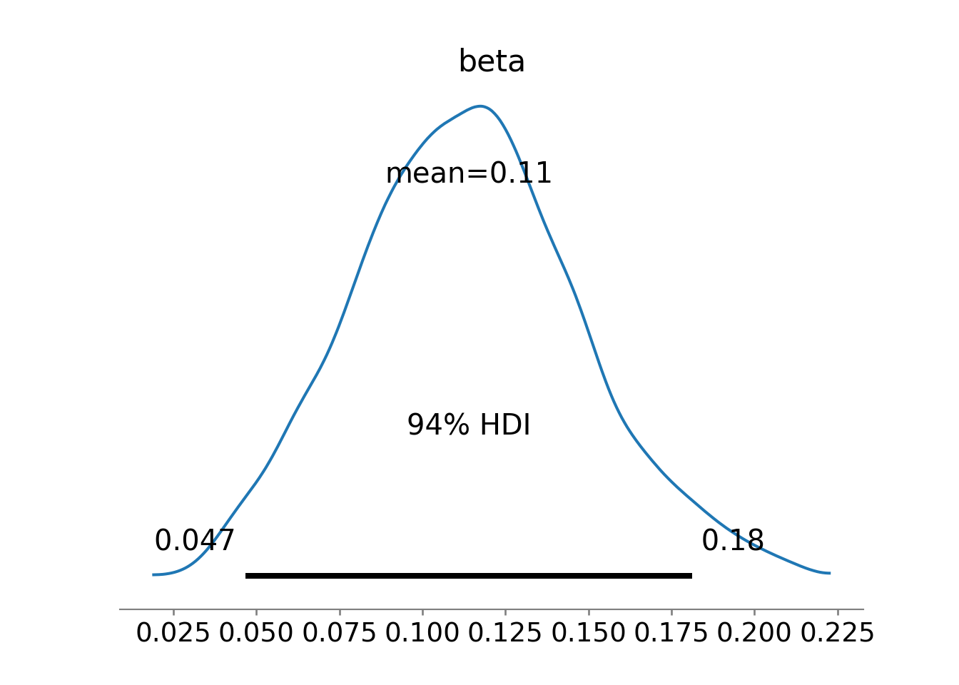
Figure 11.5 shows estimates around 0.120 are plausible, but does not clearly put the majority of plausibility above 0.120. While the estimates are most likely positive (most of the posterior density is where
(
    drawsDS
    .assign(above120 = drawsDS.beta > 0.120)
    .get("above120")
    .mean()
    .item() ## get just the value
)0.4208Yielding an approximate 43% probability for the company to at least break-even.
Interestingly, because of the uncertainty in the estimate, there is still meaningful probability that the company can earn much more than $120 per square foot, For example, here is the probability of being above $140 per square foot.
(
    drawsDS
    .assign(above140 = drawsDS.beta > 0.140)
    .get("above140")
    .mean()
    .item() ## get just the value
)0.2216yielding an approximate 22% probability for the company to earn over a very favorable $140 per square foot.
Please note that many more factors influence home price than just square footage. This model is purely for education purposes and a more detailed generative DAG to include more factors driving real-estate prices is beyond the scope of this book. Please know that you are given the building blocks to pursue that DAG if you choose.
In conclusion, there is still alot of uncertainty in the estimate of
11.2 Adding Robustness
When modelling, assumptions should reflect the reality you are trying to model. Use care traversing the business analytics bridge from real-world to math-world. For example, when it comes to housing prices, there might be alot of outliers in your data. Hence, it might be better to say that housing prices are
11.3 Explanatory Variable Centering
There are always mathematical tricks to do something a little better. In this book, we mostly shy away from the tricks to focus on the core creation process of generative DAGs and the unification of narrative, mmath, and code. However, as you advance in your journey of Bayesian modelling, you’ll see models leveraging tricks as if they are common knowledge. One such trick is explanatory variable centering.
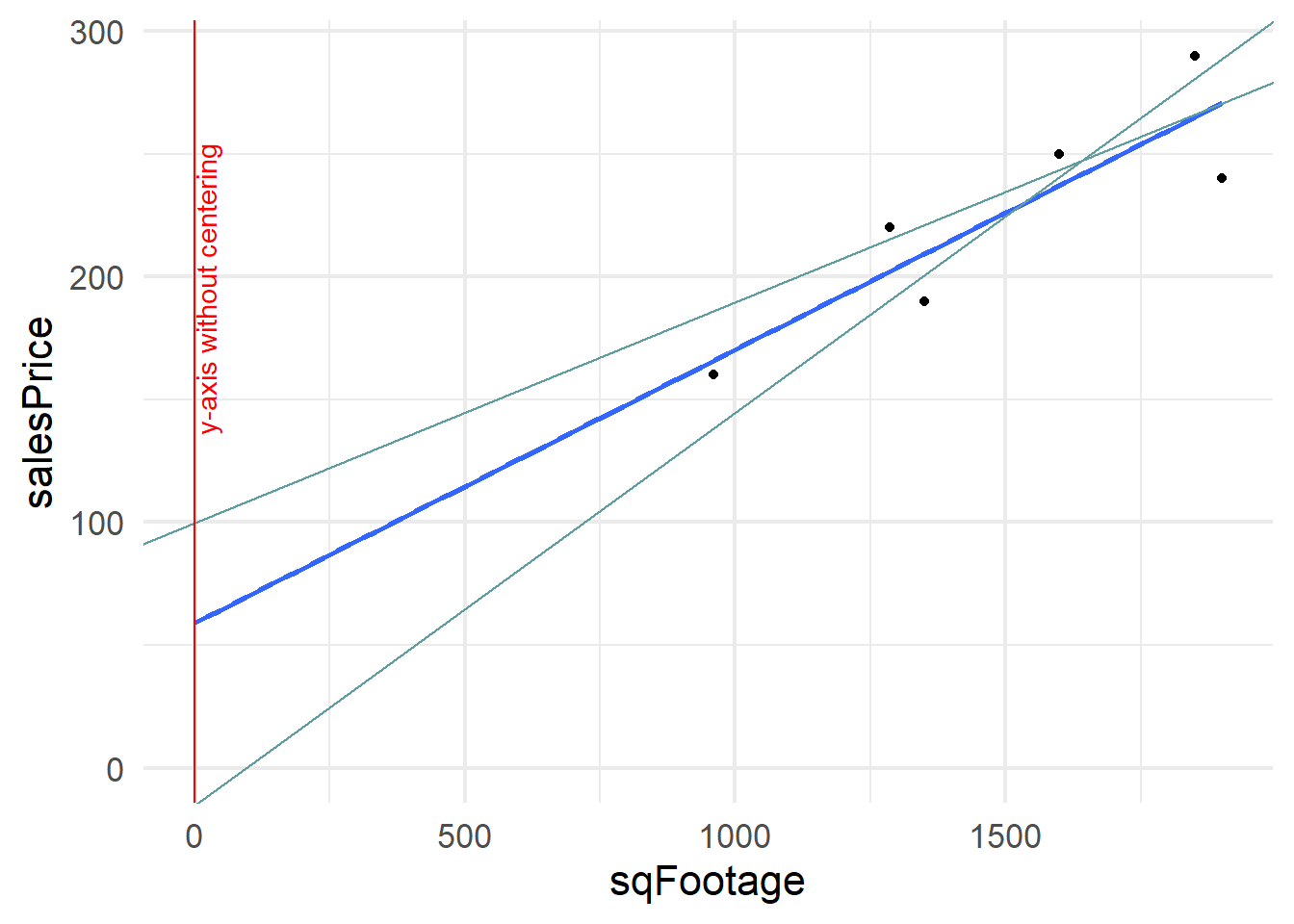
The trick we will use now is centering an explanatory variable. Figure 11.7 expands the regression line shown in Figure 11.2 to show the y-intercept at the point (0,58.9). Two other lines that plausibly describe the data are shown for comparison of with their y-intercetps. Notice the wild swings in intercepts of these lines. We captured knowledge about these wild swings with our prior knowledge
If we were to transform our square footage variable
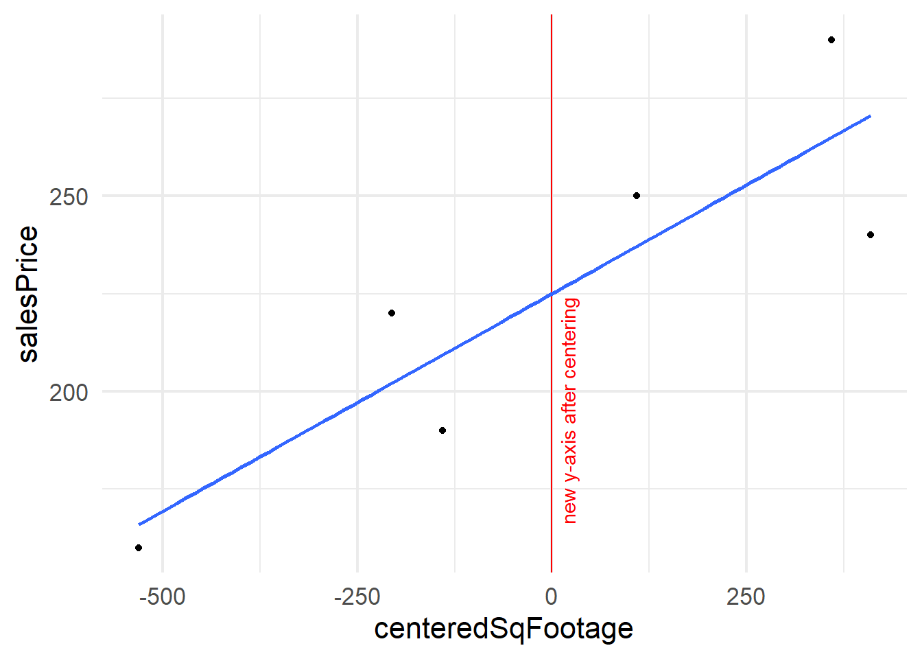
By centering the Square Footage variable, we are effectively shifting the y-axis to be drawn in the middle of our Square Footage data,
11.3.1 Notes on thinking like a Bayesian
More generally, please start to think of Bayesian models as things you, as a Business or Data Analyst, get to create. As long as you are mimicking reality with your models, you will find great success taking the building blocks you know and building models of increasing complexity that capture further nuances of the real-world. These models are yours to build - go boldly and make tailored models of the world you work in!
11.4 Getting Help
Richard McElreath’s course uses Stan instead of numpyro, yet outside of the computational engine, the material is relevant to your study. I highly recommend his lesson on linear models (see https://youtu.be/0biewTNUBP4). If you have the time, watch from the beginning. If you want to zero in on the simple linear model, he creates the first linear model trying to predict height as a function of weight at 43:00. Also, Richard McElreath’s book, Statistical Rethinking, should be the next book you buy, even though the model’s are Stan-based, tranlations of all models in the text to NumPyro are available.
11.5 Questions to Learn From
See CANVAS.