12 Narratives Told Through Graphical Models
BankPass is an auto financing company that is launching a new credit card, the Travel Rewards Card (TRC). The card is designed for people who love to take adventure vacations like ziplining, kayaking, scuba diving, and the like. To date, BankPass has been randomly selecting a small number of customers to target with a private offer to sign up for the card. They would like to assess the probability that an individual will get a TRC card if exposed to a private marketing offer. Since they are an auto-loan company, they are curious about whether the model of car (e.g. Honda Accord, Toyota 4Runner, Ford F-150, etc.) being financed influences a customer’s willingness to sign up for the credit card. The logic is that people who like adventure travel might also like specific kinds of cars. If it is true that cars are a reflection of their owners, then the company might expand its credit card offerings to take advantage of its car ownership data.
In this chapter, we use the above story to motivate a more rigorous introduction to graphical models. We will discover that graphical models serve as compact representations of joint probability distributions. In future chapters, we use these representations to help us intelligently digest data and refine our understanding of the world we do business in.
For illustration purposes, let’s assume the above story reflects a strategy where BankPass is seeking to market credit card offerings to its auto-loan customers by aligning card benefits (e.g. travel) to a customer’s preferences. Since customer preferences are largely unknown, BankPass is curious as to whether the type of car a person owns can reveal some latent personality traits which can be used to target the right customers with the right cards. In other words, can BankPass leverage its data advantage of knowing what car people own into an advantage in creating win-win credit card offerings?
12.1 Iterating Through Graphical Models
This section’s intent is to give the reader permission to be wrong. It’s okay to not draw a perfect model when you are first attacking a problem.
12.1.1 An Initial Step
You might feel lost as to how to get started capturing the BankPass problem as a graphical model? What thought process should one have? The first thought should be to make a simple graphical model of how the real-world ends up generating your variable(s) of interest; and don’t worry about how good the model is - just get something written. Figure 12.2 represents this initial attempt.
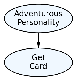
Figure 12.2 is a visual depiction of what mathematicians and computer scientists call a graph. To them, a graph is a set of related objects where the objects are called nodes and any pair of related nodes are known as an edge. For our purposes, a node is a visual depiction of a random variable (i.e. an oval) and the presence of a visible edge indicates a relationship between the connected random variables.
12.1.2 Ensuring Nodes Are RV’s
Figure 12.2 certainly conveys Bankpass’s strategy - personality will influence people’s desire to get the new credit card. However, vetting the model will reveal some shortcomings and our first vetting should be to ensure the two nodes can be modeled as random variables with each node representing a mapping of real-world outcomes to numerical values (see the “Representing Uncertainty” chapter).
For the “Get Card” node, let’s label it
Recall our goal is to represent the real-world mathematically so we can compute insight that informs real-world action.
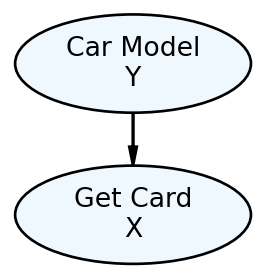
However, how do I map “Adventurous Personality” to values? In fact, what measurement or specific criteria am I using for “Adventurous Personality”? This is an ill-defined variable. Any variable we include in our models needs to be clearly defined and fulfill the requirements of a random variable; afterall, this is our key technique for representing the real-world in mathematical terms. Since the story actually suggests that Car Model is the data we have, let’s create a graphical model where Car Model helps determine the likelihood of Get Card. Using

In Figure 12.3, the difficult to measure personality node gets replaced by the car model node. To verify we can measure Car Model as a random variable, let’s be explicit about the mapping of “Car Model” outcomes to real numbers. For example:
and where
12.1.3 Interpreting Graphical Models as Joint Distributions
Mathematically, our goal is to have a joint distribution over the random variables of interest. Once we have that, we can answer any probability query we might have using marginal and conditional distributions (remember Joint Distributions Tell Us Everything). A tabular representation of the joint distribution,
| car model |
?? | |
| car model |
?? | |
| car model |
?? | |
| car model |
?? | |
| car model |
?? | |
| car model |
?? |
For all but very simple models like the one above, a tabular representation of a joint distribution becomes:
Notational Note: The use of three consecutive dots, called an ellipsis, as in these three examples: 1)
“unmanageable from every perspective. Computationally, it is very expensive to manipulate and generally too large to store in memory. Cognitively, it is impossible to acquire so many numbers from a human expert; moreover, the [probability] numbers are very small and do not correspond to events that people can reasonable contemplate. Statistically, if we want to learn the distribution from data, we would need ridiculously large amounts of data to estimate the many parameters robustly.” - Koller, Friedman, and Bach (2009)
Koller, Daphne, Nir Friedman, and Francis Bach. 2009. Probabilistic Graphical Models: Principles and Techniques. MIT press.
To overcome this, we use a different, more-compact structure - called a Bayesian Network (BN) by fancy people like computer scientists. Bayesian networks are compressed, easier-to-specify recipes for generating a full joint distribution. So, what is a BN? It is a type of graph (i.e. nodes and edges), specifically a directed acyclic graph (DAG), with the following requirements:
- All nodes represent random variables. They are drawn using ovals. By convention, a constant is also considered a random variable.
- All edges are pairs of random variables with a specified direction of ordering.
- Edges are uni-directional, they must only flow in one direction between any two nodes (i.e. directed).
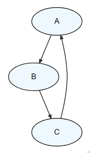
- The graph is acyclic meaning there are no cycles. In other words, if you were to put your finger on any node and trace a path following the direction of the edges, you would not be able to return to the starting node. Figure @ref(fig:acyclic) shows a cycle in a graph - it is NOT a DAG.
- Any child node’s probability distribution will be expressed as conditional solely on its parents’ values, i.e.
Let’s use Figure 12.5 to review the probability distribution implications of an edge pointing into a node (requirement 5 from above). The one edge,
12.1.4 Aligning Graphical Models With Business Narratives
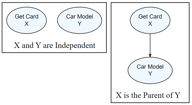
Edge presence and direction should reflect the narrative(s) your investigating. Figure 12.6 shows two alternate ways of structuring a graphical model with the same two nodes. If there are no edges between
In the next section, we will combine our models with observed data to refine our beliefs about which parameters of the DAG, if any, seem more plausible than others. More plausible parameters are essentially more plausible narratives to explain our data-generating process. This is powerful - business narratives and data analysis get linked - a generative DAG is a business analytics bridge decomposing and validating narratives to explain observed data.
12.2 Coding with Plates - The Credit Card Example

At the start of the chapter, BankPass was investigating whether prospective credit card applicants can be segmented based on the car they drove. A dataset to accompany this story is available from the web:
# ! pip install matplotlib numpyro daft --upgrade  ## then restart runtime
import pandas as pd
url = "https://raw.githubusercontent.com/flyaflya/persuasive/main/carModel.csv"
carModelDF = pd.read_csv(url)
carModelDF.head(5)
customerID carModel getCard
0 1 Toyota Corolla 0
1 2 Subaru Outback 1
2 3 Toyota Corolla 0
3 4 Subaru Outback 0
4 5 Kia Forte 1When making generative DAG’s it is helpful to start with your key or target measurement; the observed measurements that you are interested in changing by gleaming insight from your data analysis. Instead of using the prettier daft package to draw our dag’s, we will write numpyro code representing our DAG and use the more streamlined numpyro.render_model() function to visually show our DAG. Here, the measured observation we hope to improve is whether someone signs up for the credit card:
import xarray as xr
import jax.numpy as jnp
import numpyro
import numpyro.distributions as dist
from jax import random
from numpyro.infer import MCMC, NUTS
import arviz as az

# add observed data
# need jax array
getCardArray = jnp.array(carModelDF.getCard)

## define the graphical/statistical model as a Python function
def carModel():
    x = numpyro.sample('Get Card (x)', dist.Bernoulli(probs = 0.5),
                       obs = getCardArray)

## visualize using render_model() function
numpyro.render_model(carModel)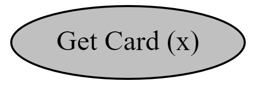
To model subsequent nodes, we consider the parameters on the right-hand side of the statistical model that remain undefined. I sneakily added a placeholder parameter of 0.5 for the probs parameter, but I only did this to show the single node model without error. In reality, this parameter is unknown and we will change it to be theta. Hence, for
In this case, we realize that Signup Probability is truly the variable of interest - we are interested in the probability of someone signing up for the card, not what car they drive. Ultimately, we want Signup Probability as a function of the car they drive, but let’s move incrementally. The below code graphically models the probability of sign-up (
def carModel():
    # theta, the parent node, must be defined before child node x
    theta = numpyro.sample('Signup Prob. (theta)', dist.Uniform(low = 0, high = 1))
    x = numpyro.sample('Get Card (x)', dist.Bernoulli(probs = theta),
                       obs = getCardArray)

## comment
numpyro.render_model(carModel)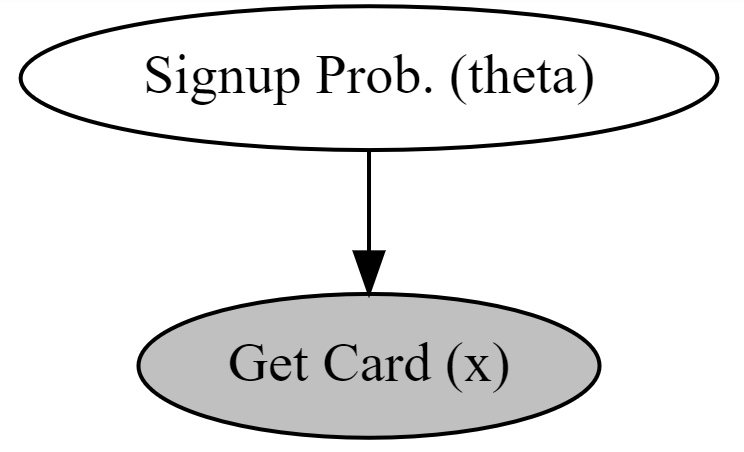
Using Figure 12.8), the generative recipe implies there is only one true
## add plate for observations

def carModel(getCardData, numObs):
    theta = numpyro.sample('theta', dist.Uniform(low = 0, high = 1))
    with numpyro.plate("i", numObs):
        x = numpyro.sample('x', dist.Bernoulli(probs = theta), obs = getCardData)

## add numObs to model_args
numObs = len(getCardArray)
numpyro.render_model(carModel, model_args = (getCardArray,numObs), render_distributions = True)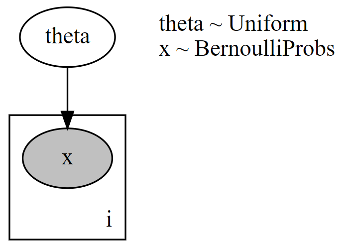
We can get the posterior distribution under this assumption:
## computationally get posterior distribution
mcmc = MCMC(NUTS(carModel), num_warmup=1000, num_samples=4000)
rng_key = random.PRNGKey(seed = 111) ## so you and I get same results
mcmc.run(rng_key, getCardArray, numObs) ## get representative sample of posterior
drawsDS = az.from_numpyro(mcmc).posterior ## get posterior samples into xarray
az.plot_posterior(drawsDS)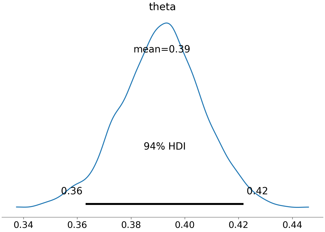

Based on Figure 12.10, a reasonable conclusion might be that plausible values for Signup Probability lie (roughly) between 36% and 42%.
12.2.1 Using pd.factorize() and Plates To Capture Narrative
Our business narrative calls for the probability to change based on car model. The plate function can then be called upon to create a generative DAG where theta will vary based on car model. A challenge in creating plates is creating indexes associated with categorical variable; for example, numpyro will not accept Toyota Corolla as a potential index. Only numbers can be used. Tackling the burden of index creation is best handled using pd.factorize() to create indexing notation.
To be as clear as possible in our communication, we switch back to showing generative DAGs created with daft.
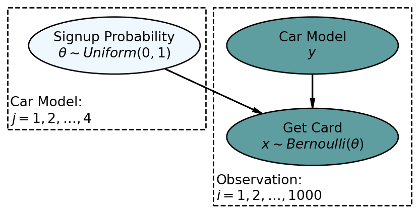
Figure 12.11 switches to zero-based indexing for the plates to be consistent with Python. Hence, the indices for the four car models will be 0, 1, 2, and 3. Let’s see how Pandas can automate index creation for us by associating each unique car model with a numeric index. We use pd.factorize on the first 20 rows of carModelDF:
pd.factorize(carModelDF.head(20).carModel)(array([0, 1, 0, 1, 2, 0, 0, 1, 0, 0, 2, 0, 3, 3, 0, 1, 0, 0, 0, 2],
dtype=int64), Index(['Toyota Corolla', 'Subaru Outback', 'Kia Forte', 'Jeep Wrangler'], dtype='object'))You can see that a two-object tuple is returned. The first object is the array of indices for car models. The second object gives the index name for each numeric index. So the index to name mapping that is created uses 0 for Toyota Corolla, 1 for Subaru Outback, 2 for Kia Forte, and 3 for Jeep Wrangler. Let’s add this id mapping (first object of tuple returned from pd.factorize()) to our car model dataframe and call it carID:
## get car model index info into data
carModelDF["carID"] = pd.factorize(carModelDF.carModel)[0] # use [0] to get data array
carModelDF["carID"]
0 0
1 1
2 0
3 1
4 2
..
995 1
996 3
997 0
998 3
999 0
Name: carID, Length: 1000, dtype: int64Using numerical indices for car model allows us to leverage numpyro’s plates to replicate Figure 12.11 in code:
Expert tip: Observed-discrete random variables, like car model, are best modeled via plates.
def carModel2(carModelData, getCardData):
    with numpyro.plate("j", len(np.unique(carModelData))) as carID:
        theta = numpyro.sample('theta', dist.Uniform(low = 0, high = 1))
    with numpyro.plate("i", len(carModelData)):
        y = numpyro.deterministic("y", carModelData)
        x = numpyro.sample('x', dist.Bernoulli(probs = theta[carModelData]), obs = getCardData)
Now, when we get the posterior distribution from our code, we get a representative sample of four
# ## computationally get posterior distribution
mcmc = MCMC(NUTS(carModel2), num_warmup=1000, num_samples=4000)
rng_key = random.PRNGKey(seed = 111) ## so you and I get same results
mcmc.run(rng_key, carModelDF.carID.values, carModelDF.getCard.values) ## get representative sample of posterior
drawsDS = az.from_numpyro(mcmc,
                coords={"carModel": pd.factorize(carModelDF.carModel)[1]},
                dims={"theta": ["carModel"]}) ## get posterior samples into xarray
az.plot_posterior(drawsDS, var_names = "theta")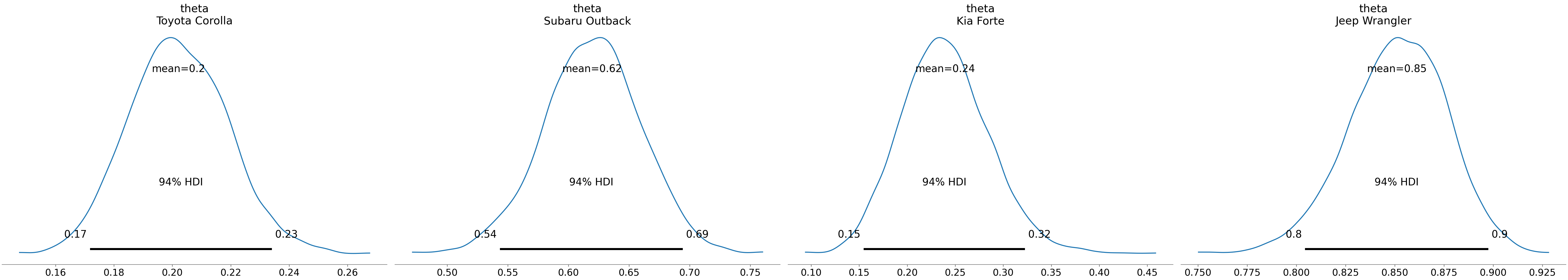
As you can see in Figure 12.12, we now have four parameter estimates. Note that we use the var_names argument to avoid having the 1,000 observations y show up in our graph. As we get better at using plates, the number of random variables we model will grow. Hence, a more compact representation of uncertainty visualization is desirable. This is accomplished with the az.plot_forest() function.
az.plot_forest(drawsDS, var_names = "theta")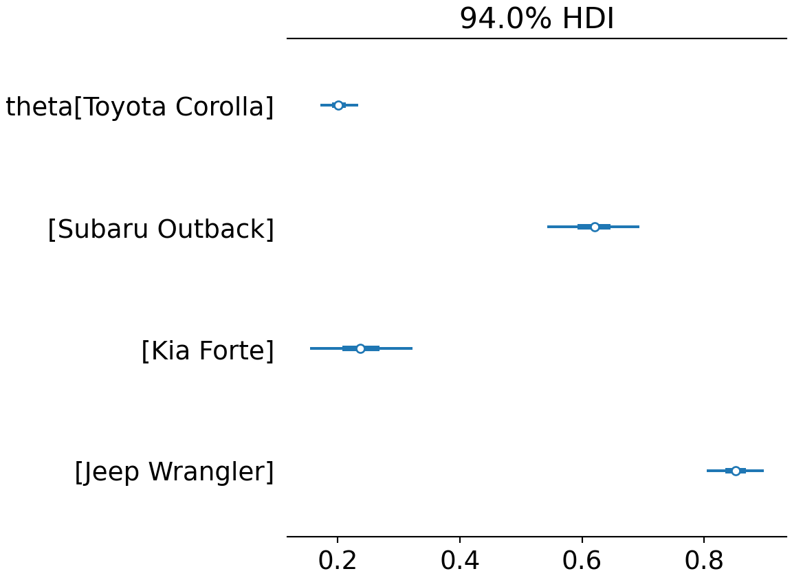
Figure 12.13 reveals almost all of the same information as Figure 12.12. We sacrifice a little bit of density shape information for being able to compactly represent all the nodes of interest.
Notice, the index names for the four theta values are automatically generated because of the coords and dims arguments passed to az.from_numpyro().
Digesting Figure 12.13, there are a couple of things to draw attention to. First, interval widths are different for the different theta values. For example, the probability interval for the Toyota Corolla is more narrow than the interval for the other cars. This is simply because there is more data regarding Toyota Corolla drivers than the other vehicles. With more data, we get more confident in our estimate. Here is a quick way to see the number of occurences of each car model across our 1,000 observations:
carModelDF.carModel.value_counts()Toyota Corolla 576
Jeep Wrangler 193
Subaru Outback 145
Kia Forte 86
Name: carModel, dtype: int64Second, notice the overlapping beliefs regarding the true sign-up probability for drivers of the Toyota Corolla and Kia Forte. Based on this, a reasonable query might be what is the probability that theta_KiaForte > theta_ToytCrll? As usual, we use an indicator function on the posterior draws to answer the question. This time though, we look at the representative sample of two random variables and recognize each row of the posterior is a realization of the joint probability distribution. So, to answer “what is the probability that theta_KiaForte > theta_ToytCrll?”, we compute:
Note: this type of query can only be answered by relying on Bayesian inference.
Also, reviewing xarray indexing practices might also be helpful here https://docs.xarray.dev/en/stable/user-guide/indexing.html.
And using this ability to make probabalistic statements, one might say “there is an approximately 77% chance that Kia Forte drivers are more likely than Toyota Corolla drivers to sign up for the credit card.
12.3 Getting Help
At this level of your training, your computational Bayesian inference questions are not easily resolved via online sources. Your best bet is to post questions - being very respectful of other people’s time - to the Pyro discussion forum. Be sure to use the numpyro tag when creating a question. Also, be sure to do a thorough search of the forum for similar questions as your question most likely has already been posed.
12.4 Questions to Learn From
See CANVAS.