
13 Linear Predictors and Inverse Link Functions
The above mosaic is put here to emphasize that we are learning building blocks for making models of data-generating processes. Each block is used to make some mathematical representation of the real-world. The better our representations, the better our insights. Instead of using Lego bricks, our tool of choice is the generative DAG. We have almost all the building blocks we need, latent nodes, observed nodes, calculated nodes, edges, plates, linear models, and probability distributions, but this chapter introduces one last powerful building block - the inverse link function.
The range of a function is the set of values that the function can give as output. For a linear predictor with non-zero slope, this range is any number from -
13.1 Linear Predictors
This chapter, we focus on restricting the range of linear predictors. A linear predictor for data observation,
where
Explanatory variable effects are fully summarized in the corresponding coefficients,
13.2 Inverse Link Functions
An inverse link function takes linear predictor output, which ranges from -
- Exponential: The exponential function converts a linear predictor of the form
- Inverse Logit (aka logistic): This function provides a way to convert a linear predictor of the form
While the beauty of these functions is that it allows us to use the easily-understood linear model form and still also have a form that is useful in a generative DAG. The downside is we lose interpretability of the coefficients. The only thing we get to say easily is that higher values of the linear predictor correspond to higher values of the transformed output.
When communicating the effects of explanatory variables that are put through inverse link functions, you should either: 1) simulate observed data using the prior or posterior’s generative recipe, or 2) consult one of the more rigorous texts on Bayesian data analysis for some mathematical tricks to interpreting generative recipes with these inverse link functions (see references at end of book).
13.2.1 Exponential Function
Figure 13.1 takes a generic example of a Poisson count variable and makes the expected rate of occurrence a function of an explanatory variable.
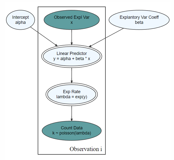
For a specific example, think about modelling daily traffic ticket in New York City. The expected rate of issuance would be a linear predictor based on explanatory variables such as inches of snow, holiday, president in town, end-of-month, etc. Since linear predictors can turn negative and the rate parameter of a Poisson random variable must be strictly positive, we use the exponential function to get from linear predictor to rate.
The inverse link function transformation takes place in the node for lambda. The linear predictor,
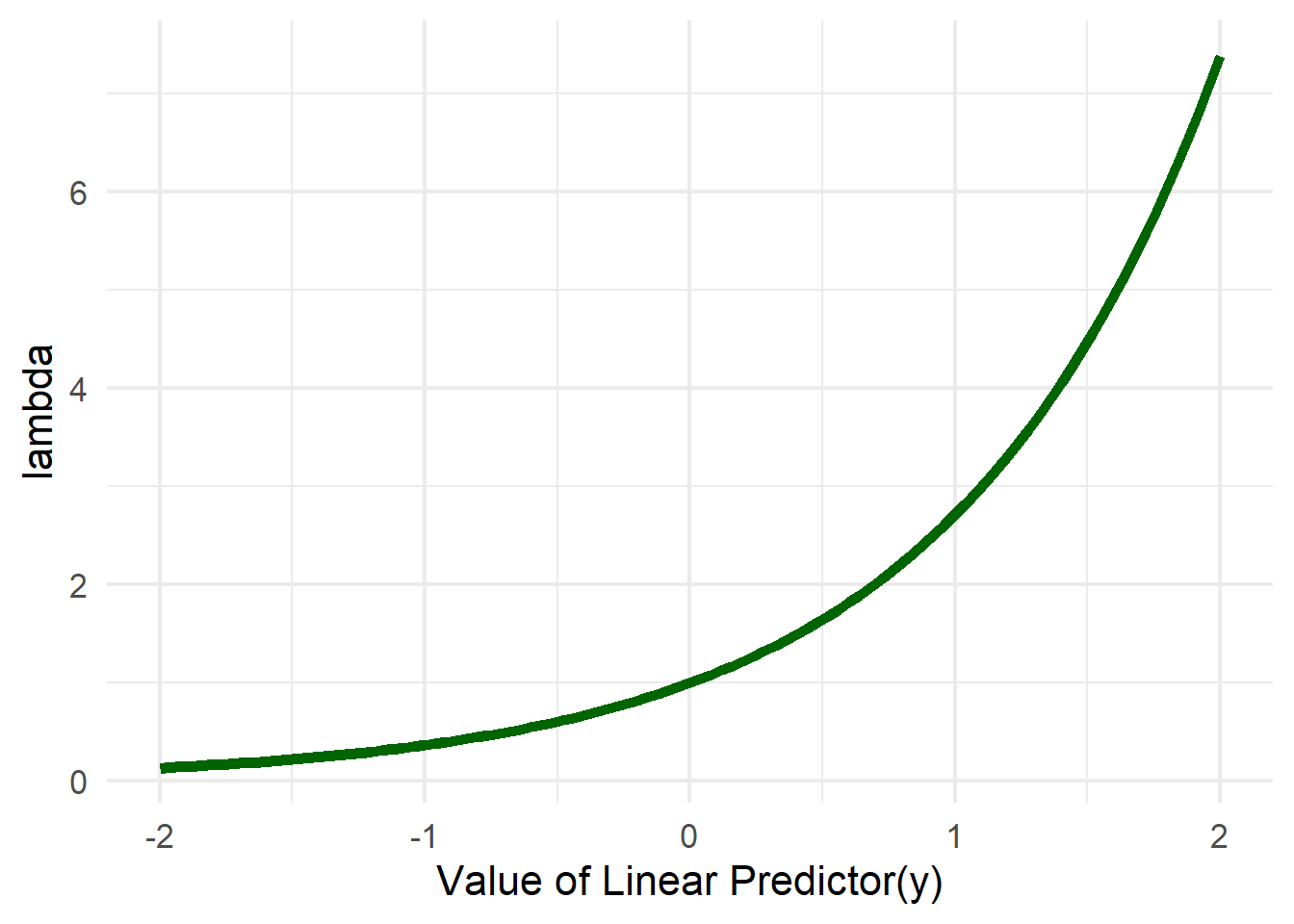
From Figure 13.2, we see that negative values of
13.2.2 Inverse Logit
Figure 13.3 shows a generic generative DAG which leverages the inverse logit link function.
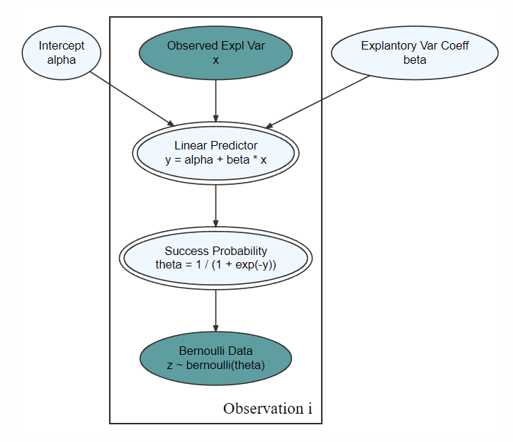
The use of the inverse logit function is done inside a method called logistic regression. Check out this sequence of videos that begin here https://youtu.be/zAULhNrnuL4 on logistic regression for some additional insight.
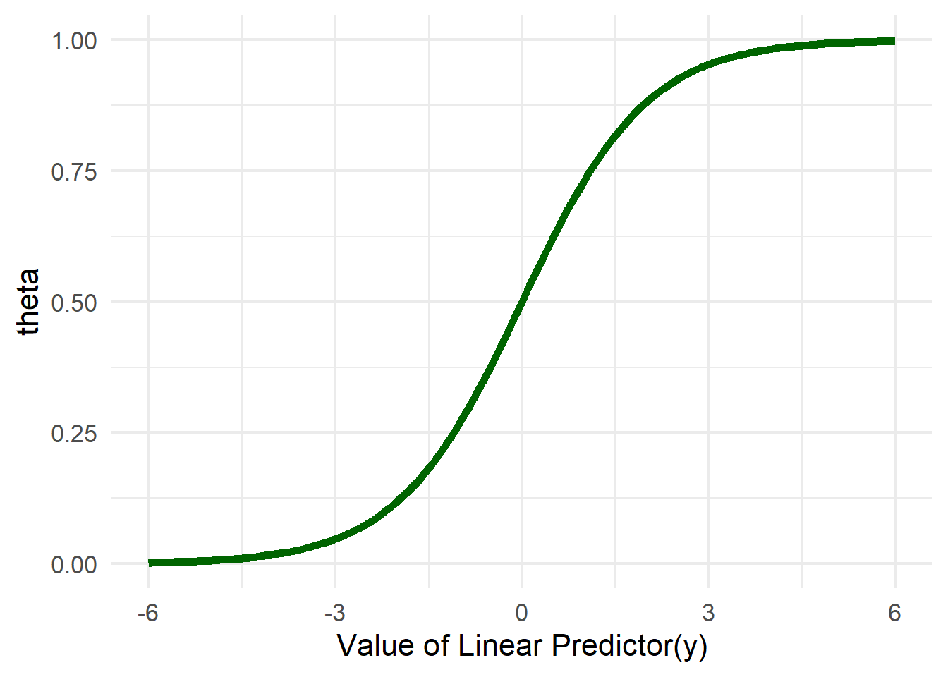
Note the inverse link function transformation takes place in the node for theta. To start to get a feel for what this transformation does, observe Figure 13.4. When the linear predictor is zero, the associated probability is 50%. Increasing the linear predictor will increase the associated probability, but with diminishing effect. When the linear predictor is increased by one unit from say 1 to 2, the corresponding probability goes from about 73% to 88% (i.e. from
13.3 Building Block Training Complete
You have officially been exposed to all the building blocks you need for executing Bayesian inference of ever-increasing complexity. These include latent nodes, observed nodes, calculated nodes, edges, plates, probability distributions, linear predictors, and inverse-link functions. While you have not seen every probability distribution or every inverse-link, you have now seen enough that you should be able to digest new instances of these things. In the next chapter, we seek to build confidence by increasing the complexity of the business narrative and the resulting generative DAG to yield insights. Insights you might not even have thought possible!
13.4 Getting Help
TBD
13.5 Questions to Learn From
See CANVAS.