15 Integration Using Monte Carlo and Markov Chain Techniques
In the previous chapters, we used representative samples of posterior distributions to answer questions using indicator functions. While we relied on these methods to make probabilistic statements, you may have wondered how and why they work. In this chapter, we delve deeper into the computational mechanisms behind Bayesian inference and explore why representative samples are critical for obtaining accurate posterior distributions in practical problems. By examining the inner-workings of integration methods and their approximations, we will actually find a deeper understanding of the underpinnings of Bayesian inference and how it enables us to make robust probabilistic statements using numpyro.
15.1 Probabilistic Statements Are Just Integrals
For the moment, let’s assume we have a concise way of representing a joint posterior distribution - let’s call this distribution \(\pi\). Recall that joint distributions allow us to map any potential set of continuous outcomes to a probability density. Closely mimicking Michael Betancourt (2019) in both notation and philosophy, let’s refer to this joint distribution’s density function as \(\pi_{\mathcal{S}}(\theta | \tilde{y})\) where any potential set of model parameters is denoted by \(\theta\), observed data is denoted by \(\tilde{y}\), and the entirety of model configuration space denoted \(\mathcal{S}\).
———. 2019. Probabilistic Modeling and Statistical Inference. https://betanalpha.github.io/assets/case_studies/modeling_and_inference.html.
When we tell narrative stories about the plausibility of potential model configurations, those stories are encoded in density \(\pi\). We then use that density to make statements about some outcome of interest. Let’s say we are interest in some function of the true generating model, let’s call it \(g(\theta)\), which could be something like profitability or some other utility function. Mathematically, the statements we make will all be in the form of expectations of some function \(g\) such the expectation is reduced to an integral over parameter space:
\[ \mathbb{E}[g(\theta)] = \int \mathrm{d}\theta\, \pi_{\mathcal{S}}(\theta|\tilde{y})\, g(\theta). \tag{15.1}\]
Integrals, like the above, cannot be evaluated analytically for most of the practical problems data analysts face, hence the data storyteller will resort to numerical methods for approximating answers to the above. The approximations will come in the form of output from a class of algorithms known as Monte Carlo methods. We introduce these methods using an illustrative example.
15.1.1 An Example Target Distribution
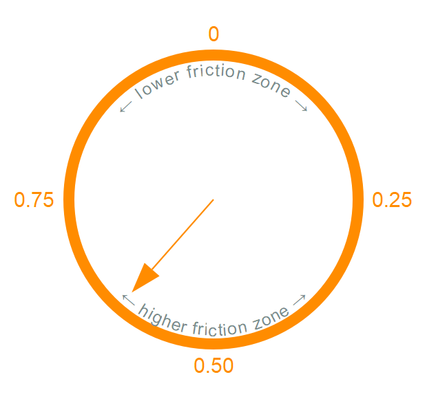
For our example, let’s imagine a game where you will win money based on the output of two random events. The first random event is that you will get a chance to spin the below spinner.
The number the spinner ends up pointing to, a decimal between 0 and 1, is your win multiplier. Let’s call it \(X\). The second random event is that each day the game organizers decide on the max win amount, \(Y\). Every contestant \(i\) for that day has a chance to win \(W_i\) dollars where \(\$W_i = X_i \times Y\). Assume you know the probability density function for the spinner:
\[ \pi_X(x) = 6x \times (1-x) \textrm{ where } x \in (0,1) \]
We graph the above density function with the following code:
import matplotlib.pyplot as plt
plt.style.use("seaborn-whitegrid")

def pi_X(x):
    if x >= 0 and x <= 1:
        return 6*x*(1-x)
    else:
        return 0

x = [i/100 for i in range(101)]
y = [pi_X(i) for i in x]

fig, ax = plt.subplots(figsize=(6, 3.5), layout='constrained')
ax.plot(x, y, color='darkblue', linewidth=4)
ax.set(xlabel=r'$x$', ylabel=r'$π_X(x)$')
ax.set_yticklabels([])

plt.show()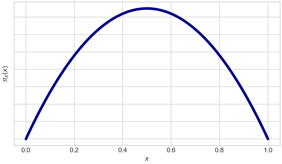
From Figure 15.2, we see outcomes near 0.5 that are associated with the “higher friction zone” shown in Figure 15.1 are truly more probable than outcomes near 0 or 1.
Additionally, let’s assume the probability density function for the day’s maximum win amount is also known:
\[ \pi_Y(y) = 2 \times 8 \times \frac{y}{10^5} \times \left(1 - (\frac{y}{10^5})^2\right)^7 \times \frac{1}{10^5} \textrm{ where } y \in (0,10^5) \]
This is actually derived from a Kumaraswamy distribution, but let’s ignore the obscure distribution name and just plot the density of \(Y\):
from matplotlib.ticker import FuncFormatter

def pi_Y(y):
    kumaRealization = y / 100000
    jacobian = 1 / 10**5
    if kumaRealization >= 0 and kumaRealization <= 1:
        return 2*8*kumaRealization*(1-kumaRealization**2)**7*jacobian
    else:
        return 0

def dollar_format(x, pos):
    """Format y-axis tick labels in dollar format"""
    return '${:,.0f}'.format(x)

x = [i for i in range(100001)]
y = [pi_Y(i) for i in x]

fig, ax = plt.subplots(figsize=(6, 3.5), layout='constrained')
ax.plot(x, y, color='darkblue', linewidth=4)
ax.set(xlabel=r'$x$', ylabel=r'$π_Y(x)$')
ax.xaxis.set_major_formatter(FuncFormatter(dollar_format))
ax.set_yticklabels([])

plt.show()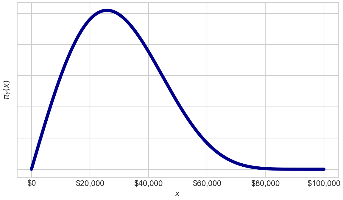
Figure 15.3 shows players can win up to $100,000, but more plausible values of max winngins are typically less than $50,000. Thus, while the game designers might advertise you can win up to $100,000 (i.e. \(X=1\) and \(Y=10^5\)), getting even close to this amount would require one to be very, very, very lucky. So a natural question at this point might be “what winnings can be expected if you get a chance to play this game?”
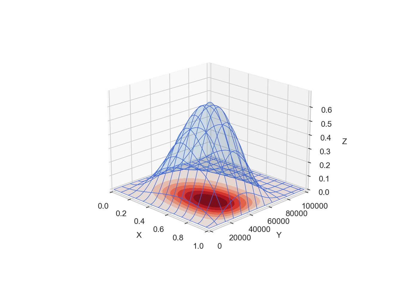
Let’s answer this by expressing the game in the language of Equation 15.1. Let \(\mathcal{S}\) be our sample space where each \(\theta \in \mathcal{S}\) can be expressed as 2-tuple of \(x \in X\) and \(y \in Y\): \[ \theta = (x,y) \] where due to the independence of \(X\) and \(Y\), the density function for \(\pi_{\mathcal{S}}(\theta) = \pi_{X,Y}(x,y) = \pi_X(x) \times \pi_Y(y)\):
\[ \begin{aligned} \pi_{X,Y}(x,y) &= 6x \times (1-x) \times 2 \times 8 \times \frac{y}{10^5} \times \left(1 - (\frac{y}{10^5})^2\right)^7 \times \frac{1}{10^5}\\ &= \frac{3xy}{3125 \times 10^5} \times (1-x) \times \left(1 - \frac{y^2}{10^{10}}\right)^7 \end{aligned} \]
The function, \(g\), that we are interested in is our winnings, \(g(x,y) = x \times y\) and our expectation of winnings:
\[ \begin{aligned} \mathbb{E}[g(x,y)] &= \int_{0}^{100000}\int_{0}^{1} \mathrm{d}x\mathrm{d}y\, \overbrace{\frac{3xy \times (1-x)}{3125 \times 10^5} \times \left(1 - \frac{y^2}{10^{10}}\right)^7\, xy}^{\textrm{Integrand: }\pi(x,y) \times g(x,y)} \\ & = \int_{0}^{100000}\int_{0}^{1} \mathrm{d}x\mathrm{d}y\, \frac{3x^2y^2 \times (1-x)}{3125 \times 10^5} \times \left(1 - \frac{y^2}{10^{10}}\right)^7 \end{aligned} \tag{15.2}\]
I do not know about you, but I see that integral and I do not want to attempt it analytically. While it’s not impossible to compute the given integral analytically, it would require significant effort and advanced mathematical knowledge. Numerical methods provide a more practical approach for obtaining an estimate of the integral. The numerical way is the easier way.
Practical Bayesian problems often involve complex models with intractable posterior distributions that cannot be computed analytically. Therefore, numerical approximation methods such as Markov chain Monte Carlo (MCMC) are commonly used to sample from the posterior and approximate the required integrals. MCMC can be computationally intensive, but it is often the most practical approach for approximating the posterior distribution in complex Bayesian models.
15.1.2 Monte Carlo Integration
One way to numrically tackle analytically-challenging integrals is to approximate them using Monte Carlo integration. Recall from calculus (or watch the below video) that an integral, like Equation 15.2, can be approximated as a summation of small regions whose total becomes a volume measurement over the region of integration.
So, thinking of Equation 15.2 as a volume of some shape, it is approximated by summing smaller shapes that consist of length \(\textrm{d}x\), width \(\textrm{d}y\), and height given by the integrand of Equation 15.2. You can see this shape in Figure 15.4.
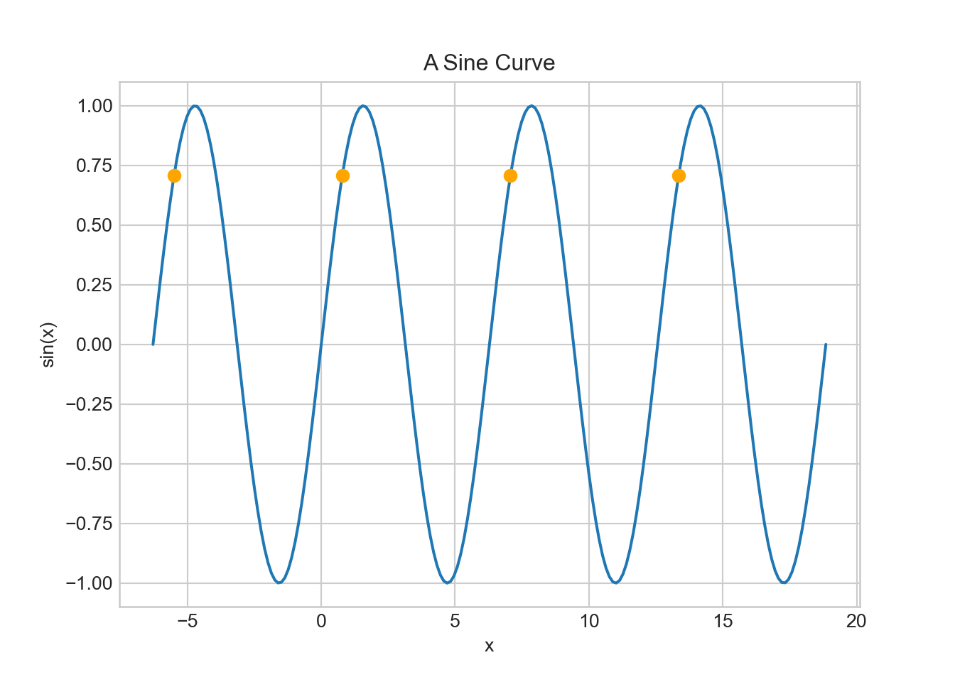
Defining \(I = \mathbb{E}[g(x,y)]\), then we can approximate \(I\) by a summation of \(N\) points randomly chosen from sample space \(\mathcal{S}\). We randomly choose the points to avoid interactions that can occur between an evenly-spaced grid and the integrand that is being estimated (e.g. imagine estimating the average value of \(\sin(x)\) by taking the evenly-spaced orange-colored sample points of Figure 15.5. Sampling \((x_1,x_2,\ldots,x_N)\) where each \(x_i \sim Uniform(0,1)\) and \((y_1,y_2,\ldots,y_N)\) where each \(y_i \sim Uniform(0,10^5)\), yields the following approximation for \(I\):
\[ \hat{I} = \frac{10^5}{N} \sum_{j=1}^{N} \frac{3x_j^2y_j^2}{3125 \times 10^5} \times (1-x_j) \times \left(1 - \frac{y_j^2}{10^{10}}\right)^7 \tag{15.3}\]
(see this article for the more general formula). Intuitively, think of each summand as the value of the integrand at a specific \(x\)-\(y\) coordinate. Averaging this value over many \(x\)-\(y\) coordinates gives the average integrand value, \(\frac{1}{N} \sum_{j=1}^{N} \frac{3x_j^2y_j^2}{3125 \times 10^5} \times (1-x_j) \times (1 - \frac{y_j^2}{10^{10}})^7\) (this is incomplete -see untitled). Since our expectation in Equation 15.2 is geometrically interpretable as a volume calculation, we multiply the area of the \(x\)-\(y\) base surface (i.e. \(10^5\)) times the average integrand value (i.e. average height) to get a volume. This volume is the answer to finding \(\hat{I}\).
In Python, we pursue \(\hat{I}\) by first obtaining the uniform grid of \(x\)-\(y\) sampling points with the below code:
import pandas as pd

N = 1000  ## sample using 1000 points

gridDF = pd.DataFrame({'winningsMultiplier': np.random.rand(N),
                       'maxWinnings': 10**5 * np.random.rand(N)})

fig, ax = plt.subplots()
ax.scatter(gridDF['winningsMultiplier'], gridDF['maxWinnings'], color='darkblue')
ax.yaxis.set_major_formatter(FuncFormatter(dollar_format))

# Set the axis labels and title
ax.set_xlabel('Winnings Multiplier')
ax.set_ylabel('Max Winnings')
ax.set_title('Randomly-Spaced Sampling Points')

plt.show()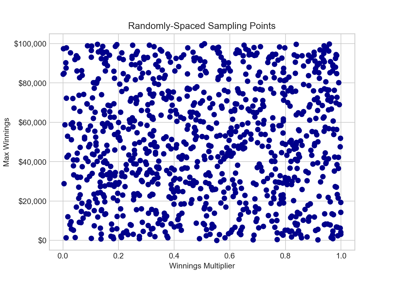
And we can then add information about evaluating the integrand of Equation 15.2 or equivalently the summand of Equation 15.3 at each of the 1,000 grid points.
# Define the integrand function
def integrandFun(x, y):
    return 3 * x**2 * y**2 / (3125 * 10**5) * (1 - x) * (1 - y**2 / 10**10)**7

# Add a column to the DataFrame using the above function
gridDF['integrand'] = gridDF.apply(lambda row: integrandFun(row['winningsMultiplier'], row['maxWinnings']), axis=1)

fig, ax = plt.subplots()
winPlot = ax.scatter(gridDF['winningsMultiplier'], gridDF['maxWinnings'], c=gridDF['integrand'], cmap='viridis')
ax.yaxis.set_major_formatter(FuncFormatter(dollar_format))

# Set the axis labels and title
ax.set_xlabel('Winnings Multiplier')
ax.set_ylabel('Max Winnings')
ax.set_title('Randomly-Spaced Sampling Points')

fig.colorbar(winPlot, label='integrand')
plt.show()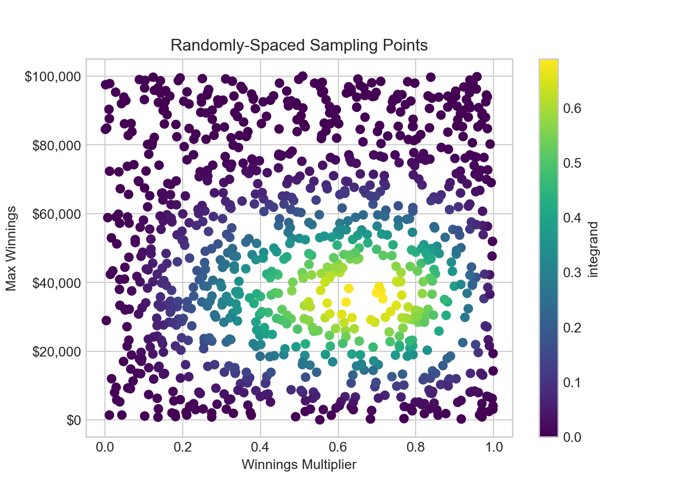
From Figure 15.7, we see that the largest contributors to \(\hat{I}\) (i.e. high integrand points) are in a sweetspot of winning multipliers near 60% - 70% and maximum winnings of around $30,000 - $40,000. These are the points that most contribute to moving the estimate of expected winnings away from zero. Points above $50,000 in maximum winnings do not contribute as much because they are improbable events. Additonally, the most probable of all the points, somewhere near 50% and $25,000, is not the largest contributor to the expectation. So it is not the largest points in terms of probability or in terms of total winnings (upper-right hand corner) that contribute the most to our expectation, rather points somewhere in between those extremes contribute the largest summands.
In code, our estimate of expected winnings turns out to be:
expectedWinnings = 10**5 * np.mean(gridDF['integrand'])
print("Expected Winnings: " + dollar_format(expectedWinnings, None))
Expected Winnings: $15,194Your calculation for expected winnings may be different than mine (i.e. due to inherent randomness in Monte Carlo integration). However, asymptotically if we were to increase \(N\), then our numbers would converge; eventually or at least after infinite samples🤷 (see the Wikipedia article on Monte Carlo integration). Here is how to see some of my randomly generated summand values - observe that highest maximum winnings does not mean largest contribution to the integrand due to the improbability of those events occurring.
gridDF.sample(n=10) winningsMultiplier maxWinnings integrand
702 0.834962 3261.267441 0.011661
204 0.019871 43354.324872 0.001626
985 0.157636 39152.398135 0.096104
739 0.794737 81238.281805 0.004317
892 0.601258 86124.118429 0.000787
261 0.969923 4789.926428 0.006133
500 0.305750 28410.414633 0.279014
850 0.038085 33348.562892 0.006526
667 0.114836 65197.370747 0.009890
143 0.750703 9848.917400 0.12219915.1.3 More Efficient Monte Carlo Integration
If the highest summands/integrands sway our expected estimates much more dramatically than all of the close-to-zero summands, then our estimation error could be reduced more efficiently if our estimation method spends more time sampling from high summand values and less time sampling at near-zero summands. One way to accomplish this is to use a non-uniform sampling of points known as importance sampling; sample the far-from-zero summands more frequently and the close-to-zero summands less frequently. In doing this, each point can no longer be weighted equally, but rather our estimate gets adjusted by the probability density function of drawing the non-uniform sample (see Wojciech Jarosz (2008)). Labelling the sampling probability density function \(g_{X,Y}(x,y)\) gives:
Wojciech Jarosz. 2008. Efficient Monte Carlo Methods for Light Transport in Scattering Media (Appendix a). https://cs.dartmouth.edu/wjarosz/publications/dissertation/appendixA.pdf.
\[ \hat{I} = \mathbb{E}_{X,Y}[f(x,y)] = \frac{1}{N} \sum_{j=1}^{N} \frac{\pi_{X,Y}(x,y) \times f(x,y)}{g_{X,Y}(x,y)} \] So instead of a uniform grid of points, I will get points in a smarter way. I will sample the winnings multiplier (\(X\)) and the max winnings (\(Y\)) using two independent truncated normal distributions that have higher density near the high integrand sweetspot, near a 0.65 winnings multiplier and $35,000 in max winnings, of the previous figure:
from scipy.stats import truncnorm

## bounds of distributions are in sd's, not actual bounds

xSamplingDist = truncnorm((0 - 0.65) / 0.3, (1 - 0.65) / 0.3, loc=0.65, scale=0.3) # winnings winningsMultiplier
ySamplingDist = truncnorm((0 - 35000) / 20000, (100000 - 35000) / 20000, loc=35000.0, scale=20000.0) # maxWinnings

# sample from the distributions
np.random.seed(123)  # for reproducibility
n = 1000  # sample size
winningsMultiplier = xSamplingDist.rvs(n)
maxWinnings = ySamplingDist.rvs(n)

integrand = integrandFun(winningsMultiplier, maxWinnings) / (xSamplingDist.pdf(winningsMultiplier) * ySamplingDist.pdf(maxWinnings))

# create a scatter plot
fig, ax = plt.subplots()
winPlot = ax.scatter(winningsMultiplier, maxWinnings, c=integrand, cmap='viridis')

# set the axis labels and title
ax.yaxis.set_major_formatter(FuncFormatter(dollar_format))
ax.set_xlabel('Winnings Multiplier')
ax.set_ylabel('Max Winnings')
ax.set_title('Non-Uniform Sampling')

fig.colorbar(winPlot, label='integrand')
plt.show()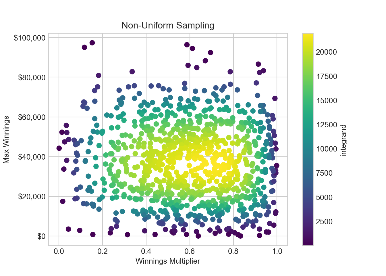
With this configuration, Figure 15.8 shows the sweetspot of x-y coordinates near 0.65 and $35,000 is now sampled much more intensely. Additionally, we see that our re-weighted integrand leads to each and every sampled point having more similar integrand values. This is a nice feature - each sample makes a more equal and significant contribution to the final estimate.
15.1.4 Estimate Sensitivity to Choice of Sampling Distribution
In the above examples of Monte Carlo integration, we approximated an integral that I was too intimidated by to attempt analytically. They gave us useful and consistent information, namely that expected winnings are in the neighborhood of $15,000 give or take a few thousand dollars. While the technique promises convergence to an exact solution, it is unclear how many samples are needed to get a level of approximation that we are comfortable with. I like to simply run the algorithms a few times and see how consistent the answers are from one run to the next. This yields an idea of how accurate the estimates might be.
# comparison of convergence
N_values = np.arange(100, 5000, step=50)

sim_results = []

def integrandFun2(x, y):
    return integrandFun(x, y) / (xSamplingDist.pdf(x) * ySamplingDist.pdf(y))

for N in N_values:
    # technique 1 grid - uniform sampling
    winningsMultiplier = np.random.rand(N)
    maxWinnings = 10**5 * np.random.rand(N)
    integrand_unif = integrandFun(winningsMultiplier, maxWinnings)
    expWinnings_unif = 10**5 * np.mean(integrand_unif)
    sim_results.append((N, 'uniform', expWinnings_unif))

    # technique 2 grid - importance sampling
    x_samples = truncnorm.rvs((0 - 0.65) / 0.3, (1 - 0.65) / 0.3, size=N, loc=0.65, scale=0.3)
    y_samples = truncnorm.rvs((0 - 35000) / 20000, (100000 - 35000) / 20000, size=N, loc=35000, scale=20000)
    integrand_imp = integrandFun2(x_samples, y_samples)
    expWinnings_imp = np.mean(integrand_imp)
    sim_results.append((N, 'importance', expWinnings_imp))

# plot the results
fig, ax = plt.subplots()
for label in ['uniform', 'importance']:
    x, y = zip(*[(N, expWinnings) for N, method, expWinnings in sim_results if method == label])
    ax.plot(x, y, label=label, marker='o')

ax.set_xlabel('N')
ax.set_ylabel('Expected Winnings')
ax.set_title('Sampling Technique Convergence - Importance Sampling is Faster')
ax.set_ylim(14000, 16000)
ax.yaxis.set_major_formatter(dollar_format)
ax.legend()
plt.show()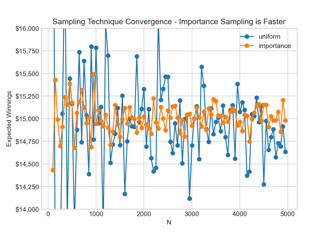
As seen from the above figure, as we increase the number of sample points, \(N\), both uniform sampling and importance sampling get more consistent approximations of estimated winnings. Notice that the yellow lines of importance sampling show less variance due to the more efficient sampling. Want even more exact answer? Say one that seems to be within a few dollars of the true integral value. One way to do this is to take a larger \(N\). Taking, say \(N=1,000,000\), I can narrow the range of estimates that I get for expected winnings to be between $14,968 and $14,987; a much narrower interval!
15.2 Sampling Efficiency
As one gets to higher dimensional problems, beyond two variables like \(X\) and \(Y\), sampling efficiency becomes critical to getting reasonable integral estimates in a finite amount of time. For most mildly complex problems, the rate of asymtpotic convergence for any estimate becomes prohibitively slow when using plain-vanilla Monte Carlo integration. In our quest for greater sampling efficiency, we will now look at two other sampling techniques belonging to a class of algorithms known as Markov-Chain Monte Carlo.
Recall the integral we want to approximate has a value accumulated over a volume of probability space \(dq\), and whose integrand is the product of probability density function \(\pi(q)\) and the function whose expected value we are trying to estimate \(f(q)\):
\[ \mathbb{E}_{\pi(Q)}[f] = \int_{\mathcal{Q}} dq\, \pi(q)\, f(q). \]
Where the expectation \(\mathbb{E}_{\pi(Q)}[f]\) of \(f\) over probability density \(\pi(q)\) is made more explicit via the underscript to the expectation operator.
When using importance sampling to approximate this integral, we made a grid of points using probability density \(g(q)\) and that allows for the approximation of the integral using the final equation shown here:
\[ \begin{aligned} \mathbb{E}_{\pi(Q)}[f] &= \int_{\mathcal{Q}} dq\, \pi(q)\, f(q) \\ &= \int_{\mathcal{Q}} dq\, \frac{\pi(q)\, f(q)}{g(q)}\, g(q)\\ &= \mathbb{E}_{g(Q)}[\frac{\pi(q)\, f(q)}{g(q)}]\\ &\approx \frac{1}{N}\sum_{i=1}^{N} \frac{\pi(q_i)\, f(q_i)}{g(q_i)} \end{aligned} \]
where \(N\) points are sampled from density \(g(Q)\). Note this trick to sample from \(g(Q)\) instead of \(\pi(Q)\) is invoked because a typical problem tends to leave us without an easy method to sample directly from \(\pi(Q)\).
Previously, we used Monte Carlo integration which is equivalent to plugging a uniform \(g(Q)\) over the volume of our spinner example into the formula above. Likewise, we used two truncated normal distributions to sample from the \(g(Q)\) density function when doing importance sampling. In Figure 15.9, we saw that the importance sampling outperformed the uniform sampling in efficiency as it converged faster.
The mathematical ideal is to minimize the variance, denoted \(\sigma^2[\cdot]\), of our approximated expectation \(\mathbb{E}_{\pi(Q)}[f]\). Let’s use some mathematical manipulation to see how the choices we make in terms of \(N\) and \(g(Q)\) affect the variance of our estimator (smaller variance \(\rightarrow\) quicker sampling):
\[ \begin{aligned} \sigma^2\left[\mathbb{E}_{\pi(Q)}[f]\right] &= \sigma^2\left[\frac{1}{N}\sum_{i=1}^{N} \frac{\pi(q_i)\, f(q_i)}{g(q_i)}\right] \\ &= \frac{1}{N^2}\sum_{i=1}^{N} \sigma^2\left[\frac{\pi(q_i)\, f(q_i)}{g(q_i)}\right]\\ &= \frac{1}{N}\sigma^2\left[\frac{\pi(q)\, f(q)}{g(q)}\right] \end{aligned} \]
where the first simplification step is due to drawing independent samples of \(q\) so that the variance of a sum is the sum of the indiviudal variances; and the second step is possible because each and every one of the \(N\) draws, i.e. each \(q_i\), is identically distributed.
The math reveals insight to reduce our estimator variance. Either we increase \(N\), or we strive to choose a \(g(q)\) that makes \(\frac{\pi(q)\, f(q)}{g(q)}\) as close to uniform as possible so that \(\sigma^2\left[\frac{\pi(q)\, f(q)}{g(q)}\right] \rightarrow 0\). Each of those approaches has a downside. Increasing \(N\) leads to increased sampling time which can get prohibitively long for complex problems. Choosing \(g(Q)\) so that \(\frac{\pi(q)\, f(q)}{g(q)}\) is uniform is also an issue because \(\pi(q)\) is usually some intractable function and making \(g(q) \propto \pi(q) \times f(q)\) is even harder. What to do?
15.3 Markov Chain Monte Carlo
Since our goal is speed, we need to aim for sampling from \(g(Q)\) so that we get a uniform value for \(\frac{\pi(q)\, f(q)}{g(q)}\). While this goal is ideal when you have one function \(f\) of critical interest, customizing the sampling method \(g(Q)\) for each function of interest will require repeated adjustment; and this adjustment is often a challenge. So for both mathematical tractability and applied pragmatism, a very popular approach called Markov Chain Monte Carlo (MCMC) seeks a slightly simpler goal; find a \(g(q)\) to sample from that yields samples from \(g(q)\) indistinguishable from samples of \(\pi(q)\).
Michael Betancourt (2018) justifies this simplification well:
Michael Betancourt. 2018. Towards a Principled Bayesian Workflow (RStan). https://betanalpha.github.io/assets/case_studies/principled_bayesian_workflow.html.
“In practice we are often interested in computing expectations with respect to many target functions, for example in Bayesian inference we typically summarize our uncertainty with both means and variance, or multiple quantiles. Any method that depends on the specifics details of any one function will then have to be repeatedly adjusted for each new function we encounter, expanding a single computational problem into many. Consequently, [we assume] that any relevant function of interest is sufficiently uniform in parameter space that its variation does not strongly effect the integrand.”
15.3.1 The Mathematical Tricks Used in MCMC
The key idea, widely used in practice, is to get \(N\) samples drawn from density \(g(q)\) so that as \(N\) gets large those samples become indistinuishable from a process using \(\pi(q)\) to generate independent samples. If done properly, this idea allows one to vastly simplify the estimation of \(\mathbb{E}_{\pi(Q)}[f]\):
\[ \begin{aligned} \mathbb{E}_{\pi(Q)}[f] &\approx \frac{1}{N}\sum_{i=1}^{N} \frac{\bcancel{\pi(q_i)}\, f(q_i)}{\bcancel{g(q_i)}}\\ & \approx \frac{1}{N}\sum_{i=1}^{N} f(q_i) \end{aligned} \]
where to estimate \(\mathbb{E}_{\pi(Q)}[f]\) one plugs in the \(N\) samples of \(q_i\) into \(f(q)\). In data-storytelling, each \(f(q_i)\) can be thought of as a real-world measurement of interest, like revenue or number of customers, and therefore, each draw of \(f(q_i)\) represents an equally likely outcome of that measurement; albeit with more draws concentrating around \(f\) values of higher probability.
The most-notable class of algorithms that support getting samples from \(g(q)\) which are indistinguishable from samples from \(\pi(q)\) directly are called Markov Chain Monte Carlo (MCMC) algorithms and they have a neat history stemming from their role simulating atomic bomb reactions for the Manhattan project. The first appearance of the technique in academia is now referred to as the Metropolis algorithm Metropolis et al. (1953) with more general application lucidly explained in Hastings (1970).
Metropolis, Nicholas, Arianna W Rosenbluth, Marshall N Rosenbluth, Augusta H Teller, and Edward Teller. 1953. “Equation of State Calculations by Fast Computing Machines.” The Journal of Chemical Physics 21 (6): 1087–92.
Surprisingly, the algorithms that approximate drawing independent samples from \(\pi(q)\) actually construct correlated or dependent samples of \(q\). The samples are drawn sequentially where each subsequent point \(q_{i+1}\) is drawn using a special stochastic (probabilistic) function of the preceding point \(q_i\). Let’s call this special function the transition function, notated by \(\mathbb{T}\), and the sequence of points is a type of Markov chain. (More generally, Markov chains are sequences of points where the next state is specified as a probablistic function of solely the current state- see here.)
The algorithms yield samples as if they were drawn from \(\pi(q)\) as long as one uses a properly constructed transition function \(\mathbb{T}(q)\) and has access to a function proportional to the desired density, let’s still call this \(g(q)\) even though it represents an unnormalized version of the normalized \(g(q)\) referred to in (?4?); both are used for generating sampling distributions. The prototypical example of \(g(q)\) is an unnormalized Bayesian posterior distribution where \(\pi(q)\) is the normalized distribution of interest.
A properly constructed transition function \(\mathbb{T}(q)\) is most easily created by satisfying two conditions (note: there are other ways to do this outside of our scope) :
- Detailed Balance: The probability of being at any one point \(q_i\) in sample space and transitioning to a different point \(q_{i+1}\) in sample space must equal the probability density of the reverse transition where starting from \(q_{i+1}\) one transitions to \(q_i\). Mathematically, \(\, \, \, \, g(q_{i}) \, \mathbb{T}(q_{i+1}|q_i) = g(q_{i+1}) \, \mathbb{T}(q_{i}|q_{i+1})\).
- Ergodicity: Each sample \(q\) in the chain is aperiodic - the chain does not repeat the same \(q\) at fixed intervals; and each possible sample \(q\) is positive recurrent - given enough samples, there is non-zero probability density of any other \(q\) being part of the chain.
Hastings (1970) then tells us to separate the transition density \(\mathbb{T}\) into two densities, a proposal density \(\mathbb{Q}\) and an acceptance density \(a(q'|q)\), to make it easy to satisfy the detailed balance requirement. Assuming a symmetric proposal density \(\mathbb{Q(q' \vert q)} = \mathbb{Q(q \vert q')}\), the following algorithm, known as random walk Metropolis, ensures the Markov chain is constructed to satisfy the requirement of detailed balance:
Hastings, W Keith. 1970. “Monte Carlo Sampling Methods Using Markov Chains and Their Applications.”
- Pick any starting point \(q_1\) from within sample space \(Q\).
- Propose a point \(q'\) to jump to next using a proposal distribution \(\mathbb{Q}(q'|q)\). This is commonly a multivariate normal distribution: \(\mathbb{Q}(q'|q) = \textrm{Normal}(q' | q,\Sigma)\).
- Calculate the acceptance probability of the proposed jump using the Metropolis acceptance criteria, \(a(q'|q) = \min(1,\frac{\mathbb{Q}(q|q) \, g(q')}{\mathbb{Q}(q' | q) \, g(q)})\), where if the proposal distribution is symmetric, simplifies to \(a(q'|q)= \min(1,\frac{g(q')}{g(q)})\). In words, if the proposed \(q'\) is a likelier state to be in, then go to it; otherwise, accept the proposed jump based on the ratio between the proposed point’s density and the current point’s density.
- Set \(q_{i+1}\) to \(q'\) with probability \(a(q'|q_i)\) or to \(q_i\) with probability \(1 - a(q'|q_i)\).
- Repeat steps 2-4 until convergence (to be discussed later).
15.3.2 Demonstrating the Metropolis Sampler
Recall our spinner example where want to sample a joint distribution of a winnings multiplier \(X\) and max win amount \(Y\) using their marginal density functions \(\pi\):
\[ \begin{aligned} \pi_X(x) &= 6x \times (1-x) \\ \pi_Y(y) &= 2 \times 8 \times \frac{y}{10^5} \times \left(1 - (\frac{y}{10^5})^2\right)^7 \times \frac{1}{10^5} \end{aligned} \]
where we are assuming we do not have a good way to sample from these two densities. Let \(q = (x,y)\) and we can then follow random walk metropolis using code.
15.3.3 Step 1: The Starting Point
# initial point - pick extreme point for illustration
qDF = pd.DataFrame({
    'winningsMultiplier': [0.99],
    'maxWinnings': [99000.0]
})
15.3.4 Step 2: Propose a point to jump to
from numpy.random import default_rng
rng = default_rng(54321)

rng = default_rng(123)
jumpDist = rng.multivariate_normal(np.zeros(2), np.diag([0.1**2, 200**2]))

q_current = qDF.iloc[0].to_numpy()
q_proposed = q_current + jumpDist
15.3.5 Step 3: Calculate acceptance probability
# density of q when params passed in as array
def pi_Q(q):
    return pi_X(q[0]) * pi_Y(q[1])

acceptanceProb = min(1, pi_Q(q_proposed) / pi_Q(q_current))
print(acceptanceProb)115.3.6 Step 4: Add point to chain
def addPoint(drawsDF, q_proposed, acceptanceProb):
    if np.random.binomial(1, acceptanceProb):
        drawsDF.loc[drawsDF.index[-1]+1] = q_proposed ## move to proposed point
    else:
        q = drawsDF.iloc[-1].to_numpy()
        drawsDF.loc[drawsDF.index[-1]+1] = q_current  ## stay at same point

addPoint(qDF, q_proposed, acceptanceProb)
print(qDF)
winningsMultiplier maxWinnings
0 0.990000 99000.00000
1 0.953221 98802.1757315.3.7 Unofficial Step (in between 4 & 5): Visualize the Chain
# create a scatter plot
fig, ax = plt.subplots()
ax.scatter(qDF.winningsMultiplier, qDF.maxWinnings)

# set the axis labels and title
ax.yaxis.set_major_formatter(FuncFormatter(dollar_format))
ax.set_xlabel('Winnings Multiplier')
ax.set_ylabel('Max Winnings')
ax.set_title('First Jump Using MCMC')
ax.set_xlim(0, 1)
(0.0, 1.0)ax.set_ylim(0, 100000)(0.0, 100000.0)plt.show()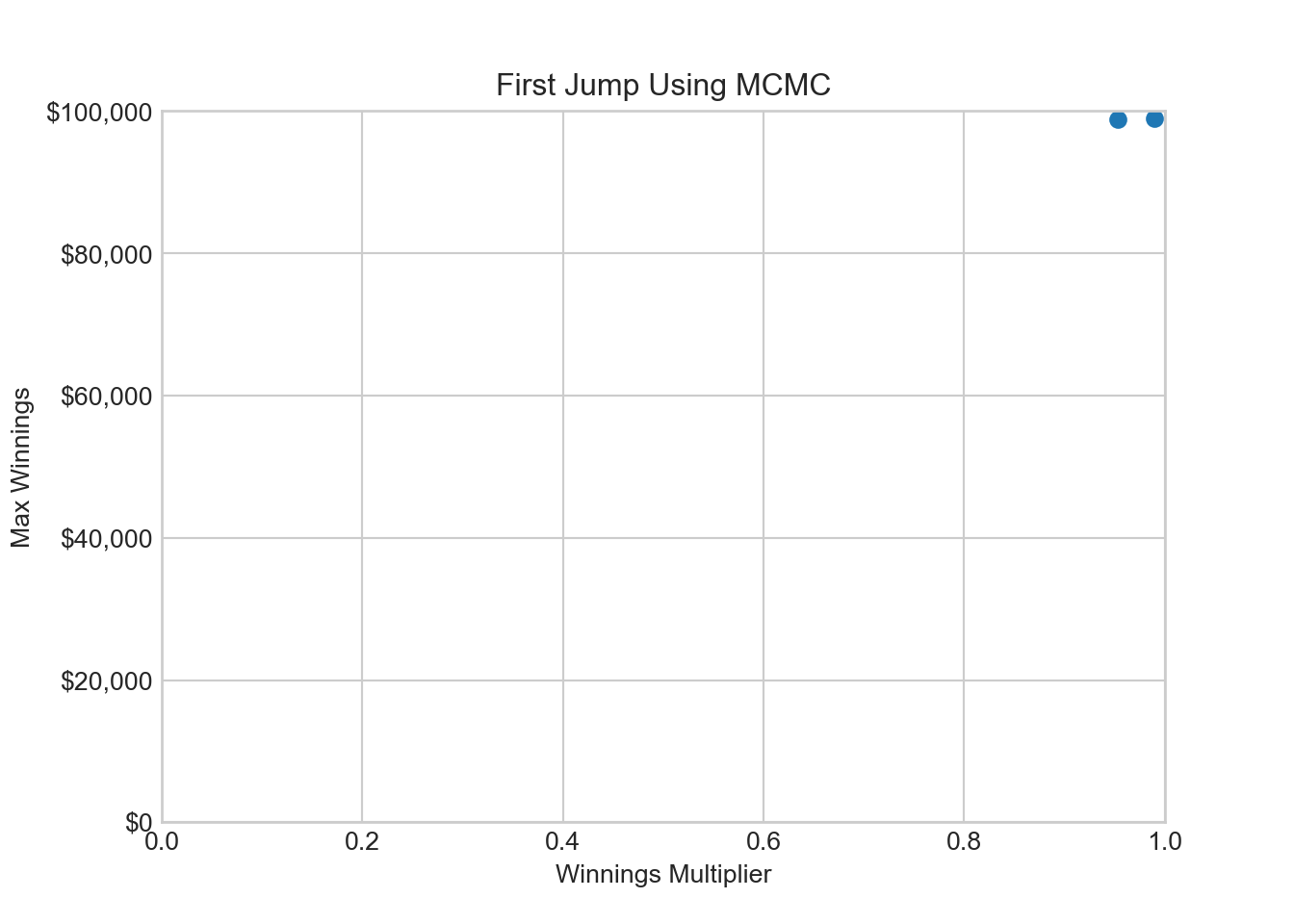
Now, those two points in the upper-right hand corner of Figure 15.10 hardly look representative of joint distribution \(Q\). Both extreme values for \(X\) and \(Y\) are highly unlikely. So while, the mathematics tells us that our sample using this Markov chain will converge to be identical to \(\pi_Q(q)\), just using two points is clearly not enough.
15.3.8 Repeat Steps 2 - 4 Until Convergence
Now, we add a function to sample more points in our chain and then gather 200 more points.
for i in range(200):
    jumpDist = rng.multivariate_normal(np.zeros(2), np.diag([0.1**2, 200**2]))
    q_current = qDF.iloc[i].to_numpy()
    q_proposed = q_current + jumpDist
    acceptanceProb = min(1, pi_Q(q_proposed) / pi_Q(q_current))
    addPoint(qDF, q_proposed, acceptanceProb)
# create a scatter plot
fig, ax = plt.subplots()
ax.scatter(qDF.winningsMultiplier, qDF.maxWinnings, s= 12, alpha = 0.4)
# set the axis labels and title
ax.yaxis.set_major_formatter(FuncFormatter(dollar_format))
ax.set_xlabel('Winnings Multiplier')
ax.set_ylabel('Max Winnings')
ax.set_title('Two Hundred Jumps Using MCMC')
ax.set_xlim(0, 1)(0.0, 1.0)ax.set_ylim(0, 100000)(0.0, 100000.0)plt.show()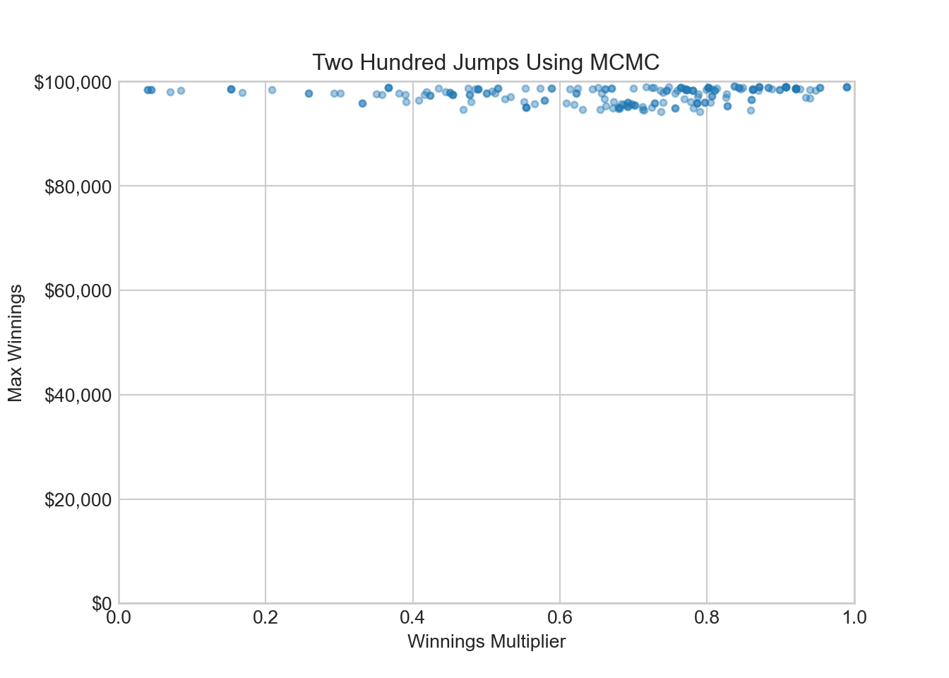
This is a fascinating plot. I will save the data associated with it as qFirstTryDF for later use.
qFirstTryDF = qDFAfter 200 jumps around parameter space, we still have not explored the sweetspot of winnings multipliers around 50% and maximum winnings around $25,000. The sample is stuck in the very flat part of the marginal density for maximum winnings \(Y\).
So far this correlated sample with its fancy Markov chain name seems like junk. What strategies can be employed so that our sample looks more like a representative sample from these two distributions?
15.4 Strategies to Get Representative Samples
15.4.1 More samples with bigger jumps
Part of the reason we are not finding the sweetspot of probability - often called the typical set - is that our exploration of \(Y\) is limited by tiny jumps. So let’s now start fresh from the same starting point, increase our jump size for maximum winnings, and take more samples.
qDF = pd.DataFrame({
    'winningsMultiplier': [0.99],
    'maxWinnings': [99000.0]
})

rng = default_rng(123)

for i in range(4000):  ## change to 4000 draws instead of 200
    ## change std dev below to 5000
    jumpDist = rng.multivariate_normal(np.zeros(2), np.diag([0.1**2, 5000**2]))
    q_current = qDF.iloc[i].to_numpy()
    q_proposed = q_current + jumpDist
    acceptanceProb = min(1, pi_Q(q_proposed) / pi_Q(q_current))
    addPoint(qDF, q_proposed, acceptanceProb)
(0.0, 1.0)(0.0, 100000.0)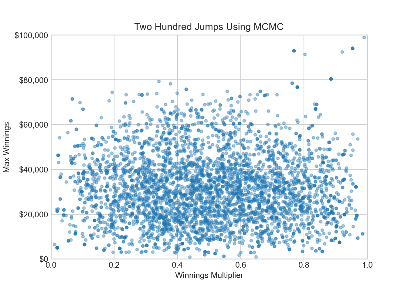
After 4,000 bigger jumps around, our sampler has unstuck itself from the low-probability density region of sample space.
15.4.2 Get rid of the burn-in period
One intuition you might have is that the starting point of your sampling should not bias your results. Think of the Markov chain as following a blood hound that visits points in proportion to their joint density magnitude. If you start the blood hound’s search in a region of very low density, then a disproportionate amount of time is spent investigating points there. To eliminate this bias, a burn-in period (say first 200 samples) is discarded and only the remaining samples are used. You can see below that discarding the first 200 points removes many points where maximum winnings samples above $60,000; we started above $60,000 and that is why there is an unrepresentatively high amount of samples from that area in the burn-in samples.
(0.0, 1.0)(0.0, 100000.0)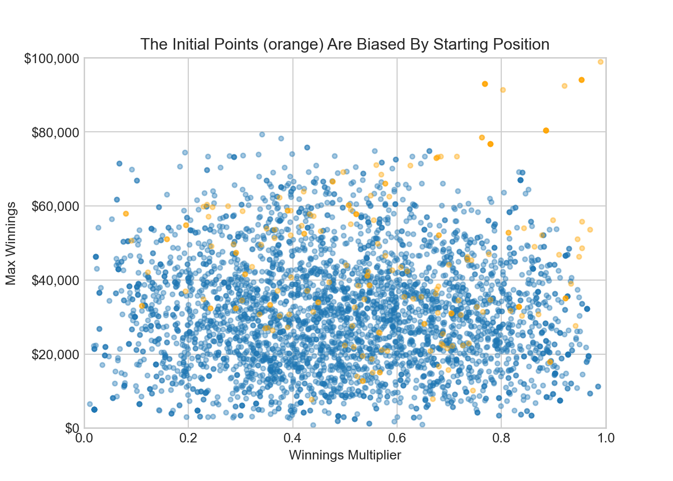
15.4.3 Thinning
One last strategy to employ is called thinning. The points are correlated by design, but if we only peek at the chain every \(N^{th}\) point, then the correlation is less detectable and samples behave more independently.
(0.0, 1.0)(0.0, 100000.0)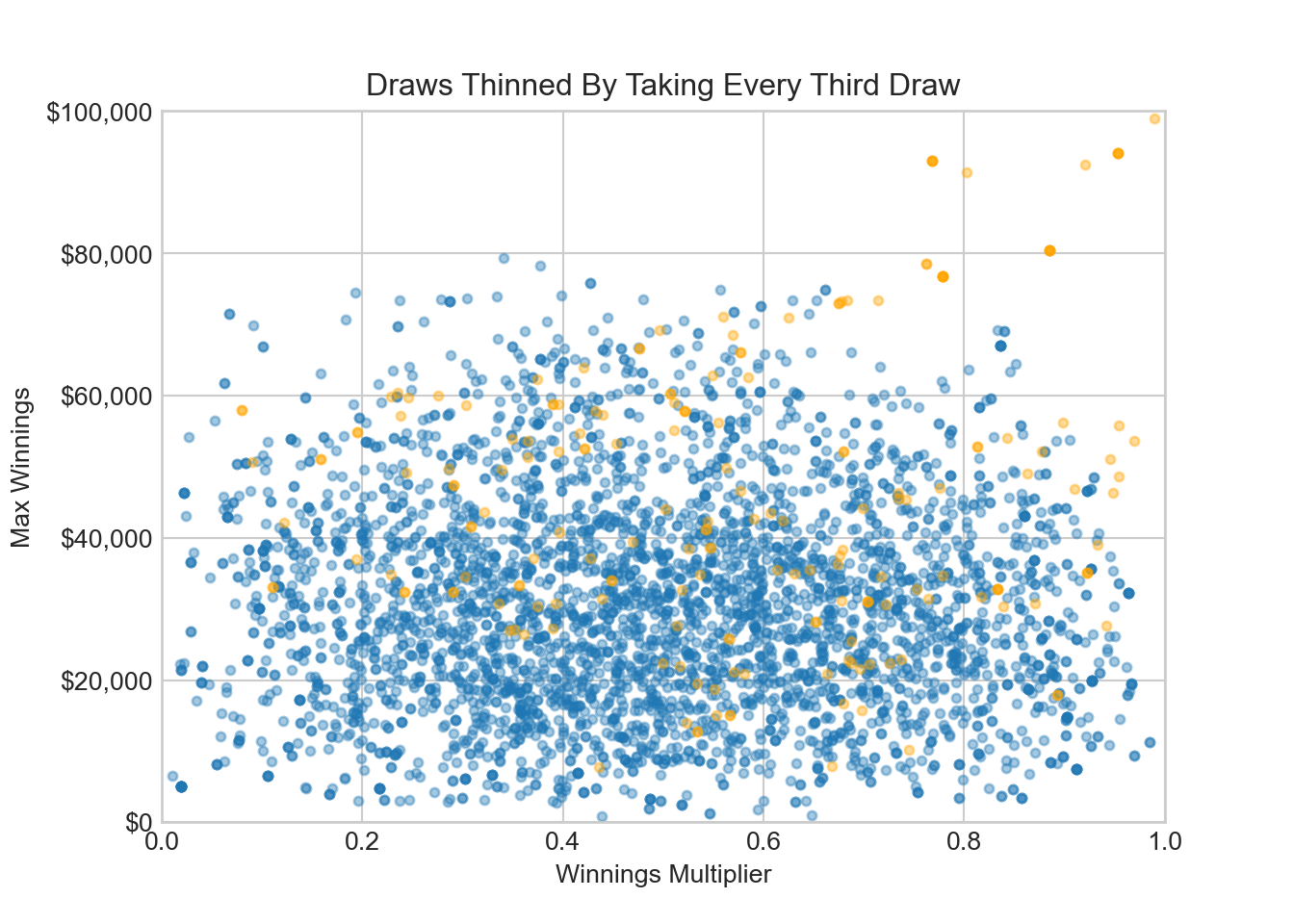
15.5 Simple Diagnostic Checks
15.5.1 Trace Plot
Recall that our goal was to estimate expected winnings. We have previously narrowed down expected winnings to be just under $15,000. Checking this on our thinned data frame sample, we find.
(qDF.winningsMultiplier[200::3] * qDF.maxWinnings[200::3]).mean()15109.227401450673Not quite the accuracy we were hoping for, but then again we only retained 600 samples. Let’s use alot more samples, say 40,000, remove the first 1,000 as burn-in, and then retain every third sample; a total of 13,000 samples.
qDF = pd.DataFrame({
    'winningsMultiplier': [0.5],
    'maxWinnings': [25000.0]
})

rng = default_rng(123)

for i in range(40000):  ## change to 40000 draws
    ## change std dev below to 1000
    jumpDist = rng.multivariate_normal(np.zeros(2), np.diag([0.1**2, 5000**2]))
    q_current = qDF.iloc[i].to_numpy()
    q_proposed = q_current + jumpDist
    acceptanceProb = min(1, pi_Q(q_proposed) / pi_Q(q_current))
    addPoint(qDF, q_proposed, acceptanceProb)

## expected winnings
(qDF.winningsMultiplier[1001::3] * qDF.maxWinnings[1001::3]).mean()15288.8086311268which is a much more accurate approximation. It is good to know this works!
One of the best ways to check that your exploring parameter space properly is to use trace plots.
For our two variables, here is a trace plot of the first 2,000 draws without removing the burn-in period.
# create a scatter plot

qDF = pd.DataFrame({
    'winningsMultiplier': [0.99],
    'maxWinnings': [99000.0]
})

rng = default_rng(123)

for i in range(2000):  ## change to 40000 draws
    ## change std dev below to 1000
    jumpDist = rng.multivariate_normal(np.zeros(2), np.diag([0.1**2, 5000**2]))
    q_current = qDF.iloc[i].to_numpy()
    q_proposed = q_current + jumpDist
    acceptanceProb = min(1, pi_Q(q_proposed) / pi_Q(q_current))
    addPoint(qDF, q_proposed, acceptanceProb)

fig, ax = plt.subplots()
ax.scatter(qDF.winningsMultiplier[200:], qDF.maxWinnings[200:], s= 12, alpha = 0.4)
ax.scatter(qDF.winningsMultiplier[:200], qDF.maxWinnings[:200], s= 12, alpha = 0.4, c = "orange")

# set the axis labels and title
ax.yaxis.set_major_formatter(FuncFormatter(dollar_format))
ax.set_xlabel('Winnings Multiplier')
ax.set_ylabel('Max Winnings')
ax.set_title('Draws Thinned By Taking Every Third Draw')
ax.set_xlim(0, 1)ax.set_ylim(0, 100000)plt.show()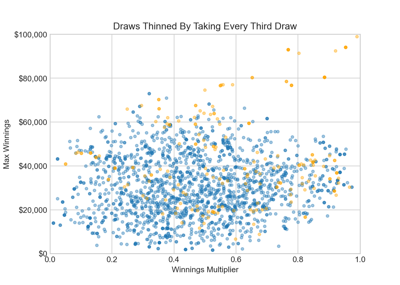
The plot shows a lack of exploration of parameter space. The bloodhound is following probability density towards the probability sweetspot, but we can tell from the plot that parameter space exploration is insufficient at this point - there is no fuzzy caterpillar, more of a worm. In our diagnostics, we will use arviz functionality to give a trace plot. You can try this code to reproduce a fuzzy caterpillar trace plot:
import numpyro
import numpyro.distributions as dist
from jax import random
import arviz as az

def model(height, weight):
    # Define priors on model parameters
    beta = numpyro.sample('beta', dist.Normal(0, 10))
    sigma = numpyro.sample('sigma', dist.Exponential(1))

    # Define likelihood of observed data
    mu = beta * height
    numpyro.sample('obs', dist.Normal(mu, sigma), obs=weight)

# Generate some fake data
true_beta = 2.5
true_sigma = 1.0
num_samples = 100
height = dist.Normal(70, 2).sample(random.PRNGKey(0), num_samples)
weight = dist.Normal(true_beta * height, true_sigma).sample(random.PRNGKey(1))

# Fit the model using MCMC
from numpyro.infer import MCMC, NUTS

nuts_kernel = NUTS(model)
mcmc = MCMC(nuts_kernel, num_warmup=500, num_samples=1000)
mcmc.run(random.PRNGKey(2), height=height, weight=weight)

# Use ArviZ to plot the trace plot of the beta parameter
az.plot_trace(mcmc.get_samples()['beta'])
15.6 Summary
In Monte Carlo integration, we use random sampling to estimate the value of an integral of a function over a given domain. The basic idea is to generate a large number of random points within the domain and use them to calculate an approximate value of the integral.
However, in many cases, generating independent random samples may not be feasible or efficient, especially in high-dimensional or complex problems where the domain of integration is large or the function being integrated is difficult to evaluate. In such cases, Markov Chain Monte Carlo (MCMC) methods can be used to generate a sequence of correlated samples from a probability distribution that is proportional to the function being integrated; .
The sequence of correlated samples generated by MCMC can be used to estimate the value of the integral, based on the Law of Large Numbers. As the number of samples in the sequence increases, the estimate of the integral becomes more accurate. Moreover, the correlation between successive samples ensures that the samples are drawn efficiently from the regions of the distribution that contribute most to the integral, leading to a more efficient estimation of the integral compared to simple random sampling.
Therefore, by using MCMC to generate a sequence of correlated samples, we can obtain a more efficient and accurate estimate of the integral compared to using independent random sampling.
15.7 Getting Help
TBD
15.8 Questions to Learn From
Exercise 15.1 Consider how you might go about adding the Kumaraswamy Distribution as a new sampler to be used with the numpyro package. This is poorly documented feature, but addressed on the numpyro discussion forum.
Your goal for this exercise is to create a new distribution, the Kumaraswamy distribution, for use with the numpyro. Write an .ipynb file demonstrating how you can create and use (small toy problem) a Kumaraswamy distribution.
Exercise 15.2 With increased problem complexity, increasing sampling efficiency or decreasing estimator variance becomes important to solving problems - like generating Bayesian posteriors - in a reasonable amount of time. To quickly get a feel for estimator variance, I will often do 20 simulation runs of \(N\) samples for a particular choice of sampling distribution \(g(x,y)\). As we did above, assume the density for \(g(x,y)\) is the product of the independent densities for \(x\) and \(y\) such that \(g(x,y) = \pi_X(x) \times \pi_Y(y)\). Now investigate the following three combinations of specifying the marginal sampling density functions:
- \(X \sim \textrm{TruncatedNormal}(0.65,0.30,0,1)\) and \(Y \sim \textrm{TruncatedNormal}(35000,20000,0,100000)\)
- \(X \sim \textrm{Uniform}(0,1)\) and \(Y \sim \textrm{Uniform}(0,100000)\)
- \(X \sim \textrm{Beta}(2,2)\) and \(\frac{Y}{10^5} \sim \textrm{Beta}(2,8)\)
Calculate the expected winnings using the assumption of the spinner game above. Do this 20 times for each of the three combinations of density functions with \(N = 10000\). For each of the three combinations, keep track of the minimum expected value and maximum expected value that is reported when running the twenty runs. Create a three row data frame reporting the results and showing the range of output (i.e. the min value and max value) returned by the three different sampling distributions. Write a comment in the code ranking the efficiency of the three different sampling distributions. Upload your code that creates this data frame as a .ipynb file.
Exercise 15.3 In proofs A.20 and A.21 of https://cs.dartmouth.edu/wjarosz/publications/dissertation/appendixA.pdf, explain what mathematical concept is being used to go from each line of the proof to the subsequent line of the proof. Upload a copy of the two proofs annotated with the mathematical concept being applied in each line as a PDF file. Example mathematical concepts include “law of total probability” or “sum of the variances equals variance of the sums for independent random variables”.
Exercise 15.4 There is code above that looks like this:
qDF = pd.DataFrame({
    'winningsMultiplier': [0.5],
    'maxWinnings': [25000.0]
})

rng = default_rng(123)

for i in range(40000):  ## change to 40000 draws
    ## change std dev below to 1000
    jumpDist = rng.multivariate_normal(np.zeros(2), np.diag([0.1**2, 5000**2]))
    q_current = qDF.iloc[i].to_numpy()
    q_proposed = q_current + jumpDist
    acceptanceProb = min(1, pi_Q(q_proposed) / pi_Q(q_current))
    addPoint(qDF, q_proposed, acceptanceProb)

## expected winnings
(qDF.winningsMultiplier[1001::3] * qDF.maxWinnings[1001::3]).mean()
It is very slow code due to the for loop. Rewrite the code using numpy arrays and vectorized functions to make it faster. Comment on the speed improvement.
Exercise 15.5 Using the notation of this chapter (e.g. \(g(\cdot),\mathbb{T}(\cdot)\), etc.), prove that the detailed balance requirement is satisfied using the proposal and acceptance densities of the algorithm above. See this Wikipedia article for the proof using different notation that applies to a finite and discrete number of sample states. Upload proof as a pdf file. (proof does not have to be extremely rigorous - this is more a lesson in transferring notation from one paper to another when notation rules are not standardized; a common task for a PhD.) I encourage you to write this up using Latex equations inside of your .ipynb file.
Exercise 15.6 In this exercise, we will explore how the choice of proposal distribution affects sampling efficiency. Specifically, create three different proposal distributions by adjusting the covariance matrix of the proposal distribution. The three distributions should represent these three scenarios:
- The Teleporting Couch Potato Scenario: The proposal distribution leads to roughly 5% of all proposed jumps being accepted.
- The Smart Explorer Scenario: The proposal distribution leads to roughly 50% of all proposed jumps being accepted.
- The Turtle Scenario: proposal distribution leads to roughly 99% of all proposed jumps being accepted.
Using a 10,000 sample chain and discarding the first 2,000 samples as burn-in, create a trace plot for winnings (i.e. winningsMultiplier * maxWinnings) for each of the three scenarios above.