3 Computational Decision Analysis

“It is rarely a mysterious technique that drives us to the top, but rather a profound mastery of what may well be a basic skill set.” ― Josh Waitzkin, The Art of Learning: A Journey in the Pursuit of Excellence

Let’s strive to master the basic skillset of decision-making by framing decision problems using three key elements:

Uncertainty: Uncertainty is our inability to know or predict a true “state of the world”. As learned in the previous chapter, we will represent uncertainty using collections of related random variables with assigned probability distributions; each plausible realization of a collection represents a “state of the world.” Our inability to know a precise state makes decision making more difficult, and makes collecting data to reduce that uncertainty more valuable.
Actions: A decision or action is an irrevocable commitment of resources that shape or restrict our possible futures. For example, signing a 1-year lease for an apartment commits your money to that type of housing; an opportunity to purchase a nearby condo may then become impossible (or at least less attractive financially in the short-term).
Objectives: An objective is a specified criteria by which preference orderings over all possible outcomes can be made. When our objective is singular and well-defined, like maximizing expected profit, we can frequently optimize our decisions. When several criteria are required for preference ordering - like using miles per gallon, cargo space, and acceleration to choose a car - things get a little trickier and we will sometimes forego optimal for simply facilitating good decisions.

These three elements: uncertainty, actions, and objectives, are foundational elements of a field known as decision theory. Combining decision theory with other concepts from mathematics, computational statistics, and data visualization will allow us to compel our stakeholders to choose strategically-aligned actions that lead to better outcomes.

Figure 3.1: A cartoon newsvendor whose business model motivates this chapter’s discussion.

Example 3.1 For this chapter, the three elements of decision analysis are demonstrated using the business model of a newsvendor (see Figure 3.1). Our newsvendor takes advantage of a single opportunity to buy newspapers every morning and then seeks to sell them on a city corner throughout the day. Our newsvendor’s goal is to match his morning purchase of papers to the demand that gets realized throughout the day. Too many papers and the newsvendor gets stuck with a pile of worthless paper; too few papers and the newsvendor misses out on profit.

3.1 Uncertainty

As discussed in Chapter 2, uncertainty is expressed using the language of random variables and assigned probability distributions. This language prominently features three key representations: 1) the graphical model, 2) the mathematical model, and 3) the computational model. The graphical model will consist of nodes and edges; one node for every random variable and edges to indicate influence of a one random variable on another. The mathematical model will be a probability distribution over the collection of random variables. Lastly, the computational model is the code required to get a representative sample of our problem.

3.1.1 Uncertainty for the Newsvendor

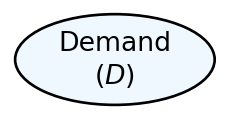
For our newsvendor (Example 3.1), the main source of uncertainty is represented as a single node for newspaper demand:

Figure 3.2: Graphical model of the newsvendor’s uncertainty.

Since we have not covered too many probability distributions, imagine a scenario where the newsvendor has access to exactly 200 potential customers and each potential customer has a 20% chance of purchase. Hence, we can now justifiably assume demand is binomial:

\[ \begin{aligned} D &\equiv \textrm{Daily demand for newspapers, and}\\ D &\sim \textrm{Binomial}(n=200,p=0.2). \end{aligned} \]

And lastly, our computational representation of demand will be a representative sample using 100 simulated draws:

Usually representative samples will require a few thousand or more draws. We stick with 100 draws here just to keep things simple.

from numpy.random import default_rng
import pandas as pd

potentialCusts = 200
purchaseProb = 0.2

rng = default_rng(seed = 111) 
numSims = 100

# create data frame to store simulated demand
newsDF = pd.DataFrame({"simNum": range(1, numSims+1),  # sequence of 1 to 100
                   "demand": rng.binomial(n = potentialCusts, 
                                          p = purchaseProb,
                                          size = numSims)})

# view first few 5 rows of newsDF
newsDF.iloc[:5,:]

   simNum  demand
0       1      42
1       2      47
2       3      43
3       4      41
4       5      38

3.2 Actions

In this book, we improve our interactions with the world by making better decisions and choosing better courses of action. These actions commit some of our resources, like time and money, to shape the plausible set of future outcomes. If we do it right, we will shift the future towards better outcomes. While we expect better results from better decisions, it is not always the case. Good decisions can have bad outcomes, like the committed toothbrusher who still gets cavities. And bad decisions can have good outcomes, like the gambler who bets his life savings on the roulette wheel and wins.

Actions feel like random variables in the sense that there is a set of alternatives to consider, the action space, that is analogous to the sample space of a random variable. However, instead of a probability distribution governing how realizations occur, we, the decision maker, get to choose which alternative from the action space is enacted.

3.2.1 Actions for the Newsvendor

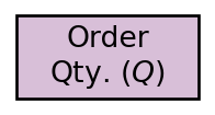
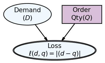
Graphically, we represent decisions using a rectangular node instead of the random-variable oval. We still provide a description of the node and shorter mathematical notation:

Figure 3.3: Graphical model of the newsvendor’s decision.

For all intents and purposes, decision nodes are random variables with a single outcome that is chosen by the decision-maker. The value of decision nodes gets passed through a graphical model in the same manner that the stochastic value of a random variable node would pass its value to its children.

For the mathematical model, we provide the set of alternatives in lieu of a random variable with assigned probability distribution:

\[ \begin{aligned} Q &\equiv \textrm{Order quantity chosen by decision-maker, where}\\ Q &\in \{0, 1, 2, \ldots, 200\}. \end{aligned} \]

where we choose our potential order quantities to be in the range of plausibly seen demand values. Let’s call the above, the discrete-choice newsvendor model.

For computational tractability (to be discussed in subsequent chapters) and for cases where fractional quantities can be represented, it is often useful to consider a continuous-choice model where:

\[ Q \in \{q | q \in \mathbb{R}, 0 \leq q \leq 200\} \]

where you interpret this set-builder notation as saying “$Q$ is in the set of all order quantities $q$ such that $q$ is a real number ($q \in \mathbb{R}$); and $q$ is between 0 and 200 (inclusive).” In simpler phrasing, order quantity $q$ can be any number between 0 and 200, even non-integers like $20.2623$ newspapers.

3.3 Objectives

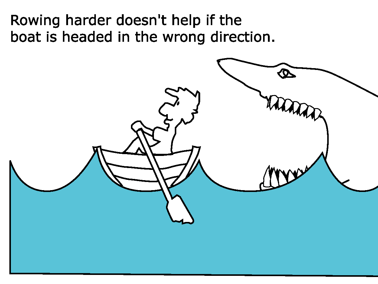
Of all the modelling assumptions we make, the most important is that of articulating objectives. Effort spent refining a decision model is wasted when objectives are poorly specified as comically depicted in Figure 3.4.

Figure 3.4: Words to live by. Quote by Kenichi Ohmae, Partner at McKinsey.

So, prior to embarking on any data-driven improvement effort, find or craft a strategy statement that serves as your navigational aid and documents your assumed objectives as an analyst (see Collis and Rukstad 2008 for one way to do this). Be vocal about this assumed strategy when talking with stakeholders; it will absolutely lead to informative and collaborative conversations. Conversely, any unaddressed misalignment between you and your stakeholders may quickly lead to your dismissal from the meeting or the company. For example, a market-share-maximizing CEO might abhor your repeated focus on minimizing production costs when they feel maximizing customer acquisition and retention are much more important than saving a penny in the production process.

Collis, David J, and Michael G Rukstad. 2008. “Can You Say What Your Strategy Is?” Harvard Business Review 86 (4).

3.3.1 Functions to Represent Objectives

When it is possible to mathematically represent our preference ordering over potential “states of the world”, we can often computationally find so-called “optimal” decisions which lead to a best possible state or outcome. Examples of single measurable states or outcomes of interest that make for easy preference ordering include profit, cost, utility, and loss where maximizing or minimizing the outcome yields an easy way to indicate preferences. In practice, however, this is often really hard; think of the challenges trying to rank cars, universities, houses or any other big decision in your life; its not as simple as saying “more profit is better”.

3.3.1.1 Utility Functions

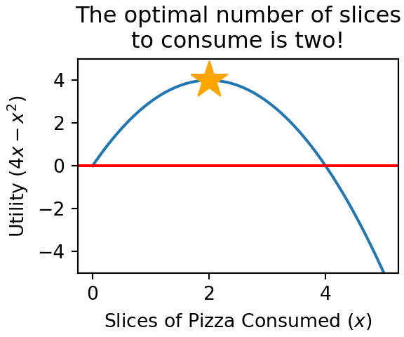
Utility functions map each potential outcome, or equivalently each potential state of the world, to a single value representing our satisfaction with that outcome; we call a quantifiable satisfaction value utility. For example, let $x \equiv \textrm{Number of pizza slices you consume}$ and a utility function be defined as $u(x) = 4x - x^2$. So, the utility of consuming one slice of pizza would be measured as 3 utils (utils is a made-up term for the unit of measure of a utility function). Plugging in values other than $x=1$, the utility of consuming two slices ($x=2$) is 4 utils, and the utility of getting sick after six slices ($x=6$) would be -12 utils. The beauty of having a utility function is that we can optimize our decision; Figure 3.5 helps us see two slices of pizza is optimal.

Figure 3.5: Plotting the utilty function for consumed pizza and noting maximum utility occurs at two slices.

3.3.1.2 Loss Functions

In other cases, a cost function might be used to represent dissatisfaction. Functions where smaller numbers are better are called loss functions; one such loss function, common in many domains including demand forecasting, is an absolute error loss function:

\[ \ell(d,q) = |(d-q)| \]

where $d$ is an observed value and $q$ is a prediction for the observation. For a newsvendor, we might interpret $d$ as some unknown demand, $q$ as the order quantity made prior to observing demand, and loss function $\ell$ as a measure of dissatisfaction with the chosen order quantity after observing $d$. Obviously, choosing $q=d$ would optimally minimize loss… unfortunately for our newsvendor, he has to pick a $q$ before observing $d$.

3.4 Choosing Optimal Actions For Specific Objective Functions

One reason we like well-defined objective functions, like loss or utility, is that we can ask the computer for help optimizing our decisions. Let’s take the pizza example in Figure 3.5 and numerically discover the optimal amount of pizza to consume. Recall,

\[ \begin{aligned} x &\equiv \textrm{Slices of pizza consumed}\\ u(x) &= 4x - x^2 \end{aligned} \]

where our goal to maximize utility by choosing among all possible continuous values of $x$,

\[ \max_{0 \leq x \leq 200} u(x) = \max_{0 \leq x \leq 200} \left(4x - x^2\right). \]

If you come across math notation that you do not understand, such as $\max_{0 \leq x \leq 200} \left(4x - x^2\right)$, just google some related terms, e.g. max math notation meaning. In this case, the second link for me led to a helpful pdf titled Argmax and Max Calculus. You might end up clicking on a few worthless links, but with practice you get better at choosing search terms and knowing which sites are helpful. math.stackexchange.com and stackoverflow.com/ are two of my favorites for math and programming help, respectively.

Certainly, for this type of function either plotting it as in Figure 3.5 or some introductory calculus will get us the optimal $x$. However, when we model the real-world, the plots and the calculus become unmanageable and we will have to rely on numerical methods. Let’s learn those methods now while things are simple and then feel like superheroes later when we use them to solve much more complicated problems.

3.4.0.1 Numerical Optimization Using Gradients

Let’s introduce the math and coding concepts behind numerical optimization by continuing our pizza example. In simple words, the steps we will take to optimize pizza eating in the computer are as follows:

Define a Utility Function: Define a mathematical function of utility given input of how many slices of pizza you will eat.
Initialize Input Values: Pick some number of slices of pizza to simulate eating.
Calculate how utility might change: Calculate how utility would change if we eat just slightly more pizza than we chose to eat in step 2.
Choose a New Input Value: If utility increases with a little more pizza, repeat steps 2 and 3 using a slightly higher simulated value of slices to eat. Similarly, if utility decreases, repeat steps 2 and 3 using a slightly lower simulated value of slices to eat.
Iterate Until Satisfied With Result: Repeat steps 2-4 until changes in utility are not practically relevant.

Now we take the narrative of the above steps, and present the corresponding math and code.

Step1 - Define a Utility Function: For step 1, we have the math complete already:

\[ \begin{aligned} x &\equiv \textrm{Slices of pizza consumed}\\ u(x) &= 4x - x^2 \end{aligned} \]

And the code (this function is visualized in Figure 3.5),

from jax import grad, vmap
import jax.numpy as jnp
import pandas as pd

## write utility function in Python
def utilityFunction(x):
    # x represents number of consumed pizza slices
    utility = 4*x - x**2   # x**2 is the square of x
    return utility

## check it works, e.g. for u(1) should = 3
print(utilityFunction(1))

which includes the importation of some functions we will use in subsequent steps.

Step2 - Initialize Input Values: We can pretty much start with any feasible value of pizza consumption. Let’s start with $x=1$ and use a data frame to capture the evolution of our simulation. In code,

simNum = 1
xValue = 1
df = pd.DataFrame({"simNum": [simNum], "x": [xValue],
                   "utility": utilityFunction(xValue)})
df

   simNum  x  utility
0       1  1        3

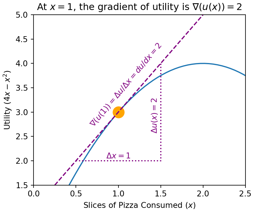
Step3 - Calculate how utility might change: The general mathematical object that defines how utility changes in response to changes in input values is called the gradient. When we have only one input variable to a function, like the $x$ in calculating $u(x)$, the gradient of that function at a given input value, say $x=1$, returns the derivative of a function at that input value (think slope of tangent line at that point). The gradient function is denoted $\nabla$(greek letter “nabla”), and the gradient at a specific point, say $x=1$, is $\nabla u(1)$ calculated as the derivative of the function at that point. So, do not be alarmed if your calculus is rusty or non-existent, that is okay, but we show the calculus approach here to demonstrate that the code will indeed emulate the math:

A function like $f(x,y,z)$ with three inputs will have a three-element gradient. Intuitively, each element can be thought of as a slope representing the change in objective function for a slight increase in the corresponding input variable. More rigorously, each element is the partial derivative of the objective function with respect to the input variable. So, the gradient of $f(x,y,z)$, denoted $\nabla f(x,y,z)$ is a three-element vector of partial derivatives:

\[ \nabla f(x,y,z) = \left[\frac{\partial f}{\partial x}, \frac{\partial f}{\partial y}, \frac{\partial f}{\partial z} \right] \]

where the gradient is shown as a row-vector for compactness, but is probably more frequently thought of as a column-vector for math computations. Don’t worry too much if this little side note scares you, we will cover the details as they are needed in subsequent material.

\[ \begin{aligned} \nabla u(x) &= \left[\frac{\partial{u}}{\partial{x}}(x)\right]\\ &= 4 - 2x \\ \implies \nabla u(1) &= 2 \end{aligned} \]

Figure 3.6: The gradient of the utilty function at any point is the slope of the tangent line at that point.

Figure 3.6 shows that at $x=1$, the derivative of the utility function with respect to slices of pizza consumed is 2, $\nabla u(x) = du/dx=2$. It means that if we are consuming one slice of pizza, we should expect to increase our utility by 2 utils for every additional slice of pizza. A positive slope indicates utility will increase with increases in the function’s input, whereas, a negative slope indicates an input variable should be decreased to yield higher utility. Studying Figure 3.6, the ratio of increased utility to increased pizza consumption is not constant and will change even for tiny fractional changes in consumption. In fact, the 2-to-1 ratio of change in utility to change in pizza only applies when we are consuming exactly one slice of pizza; at other amounts of pizza consumption, the slope is different. At $x=2$, for example, the slope of the tangent line will be zero, hence, there is no additional utility for increased consumption at that point.

The good news is that we do not have to know or remember calculus to get the slope of the utility function. Python’s jax package can calculate slopes, i.e. gradients, for us. We do that here using the grad function from the jax package:

## define gradient of u(x) (i.e. the slope)
utilityFunction_dx = grad(utilityFunction)

## show gradients (slope) at various x-values
x = 1.

## add gradient column to dataframe
gradient = utilityFunction_dx(x)
df["gradient"] = gradient.item()  ##ARGH: convert device array to scalar
df

   simNum  x  utility  gradient
0       1  1        3       2.0

The grad function takes a function as input and provides a function as output. The output function, which we assigned to utilityFunction_dx, is the gradient function we just learned about. This gradient function returns the slope of the line tangent to the function at a given point. Above, we use the new function, utilityFunction_dx(), to get the gradient of utility at x=1; note that it matches the analytic result shown in Figure 3.6.

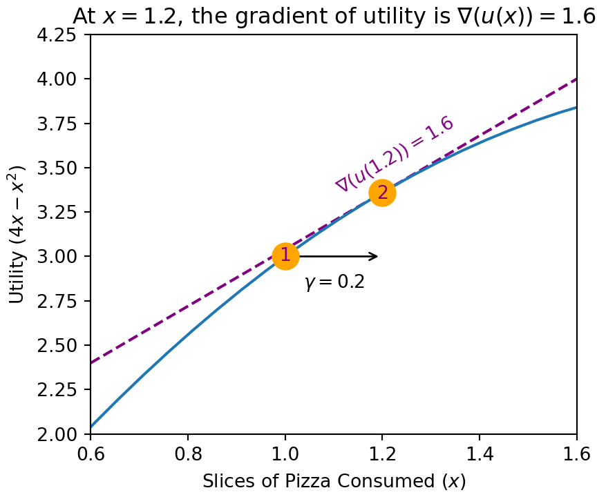
Step4 - Choose a New Input Value: Knowing that the gradient is positive at $x=1$ tell us that utility will increase if we increase $x$. We just have to decide the right step size, often notated with $\gamma$ (“gamma”), the amount we will increase $x$. Let’s set $\gamma = 0.2$ for our first step; we’ll see if eating 0.2 slices more of pizza get’s us closer to maximum utility. Skipping our typical math exposition, we jump right into code showing this step:

## increment simulation number
simNum = simNum + 1

## step size
stepSize = 0.2

## decide which x to try next
if gradient >= 0:
  xValue = xValue + stepSize
else:
  xValue = xValue - stepSize

## get variable values for new row
utility = utilityFunction(xValue)
gradient = utilityFunction_dx(xValue).item()
newRow = pd.Series({"simNum": simNum,
                    "x": xValue,
                    "utility": utility,
                    "gradient": gradient})

## Append single new row to dataframe
df = pd.concat([df, newRow.to_frame().T], ignore_index = True)
df

   simNum    x  utility  gradient
0     1.0  1.0     3.00       2.0
1     2.0  1.2     3.36       1.6

Figure 3.7 shows the result of the stepping process. We started at the orange point marked #1 where $x=1$, $u(x) = 3$, and $\nabla u(x) = 2$. Because the gradient was positive, we increased $x$ by step-size $\gamma = 0.2$ moving us to the point marked #2 at $x=1.2$, $u(x) = 3.36$, and $\nabla u(x) = 1.6$

Figure 3.7: The gradient of the utilty function at any point is the slope of the tangent line at that point.

Since the gradient at this new point remains positive, we will continue the next step by increasing the value of $x$ that we try.

Step5 - Iterate Until Satisfied With Result: From the gradient, we know our objective function can still increase, there is still a slope to “ascend the hill” and continue to increase our objective function. Let’s set a stopping criteria that if the gradient is close to zero, i.e. we are close to the top of the hill, then we will stop. We can also stop after a certain number of maximum steps to avoid putting ourselves into an infinite loop. Here is the code to keep “climbing the hill” - a process mathematicians call gradient ascent:

maxSteps = 10 ## set to avoid looping forever
for _ in range(0,maxSteps):
    ## increment simulation number
    simNum = simNum + 1

    ## decide which x to try next
    if gradient >= 0:
        xValue = xValue + stepSize
    else:
        xValue = xValue - stepSize

    ## get variable values for new row
    utility = utilityFunction(xValue)
    gradient = utilityFunction_dx(xValue).item()
    newRow = pd.Series({"simNum": simNum,
                        "x": xValue,
                        "utility": utility,
                        "gradient": gradient})

    ## Append single new row to dataframe
    df = pd.concat([df, newRow.to_frame().T], ignore_index = True)

    ## break out of for loop is gradient val is sufficiently small
    if abs(gradient) < 0.1:
        break
      
df

   simNum    x  utility  gradient
0     1.0  1.0     3.00       2.0
1     2.0  1.2     3.36       1.6
2     3.0  1.4     3.64       1.2
3     4.0  1.6     3.84       0.8
4     5.0  1.8     3.96       0.4
5     6.0  2.0     4.00       0.0

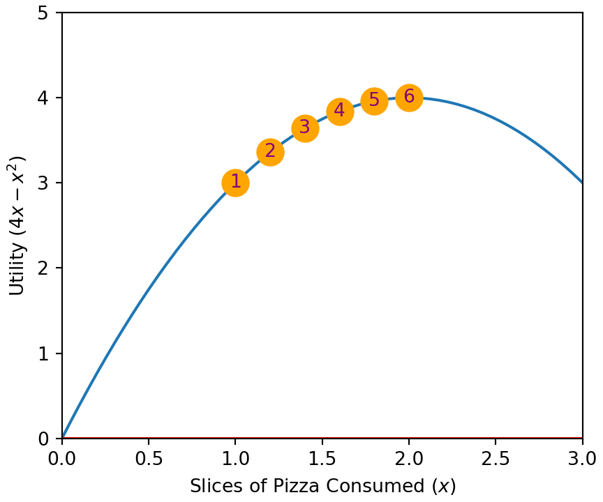
The simulation is complete after six steps, we found the top of the utility hill. Figure 3.8 shows our path, slow and steady from the point marked #1 to the point marked #6. In the exercises, we will explore more problems where the path is less smooth and further build our intuition around using gradients for optimization.

Figure 3.8: Six steps to get to the point of maximum utility.

3.5 Optimizing Actions Under Uncertainty

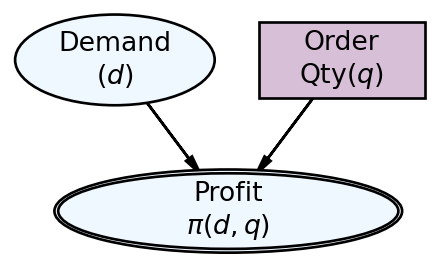
Returning to our newsvendor example, the graphical model of Figure 3.9 shows the explicit dependence of our objective function on our uncertainty about demand and our decision on how much to order.

Figure 3.9: Graphical model of the newsvendor’s decision model.

The statistical model accompanying Figure 3.9 is shown here:

\[ \begin{aligned} D &\equiv \textrm{Daily demand for newspapers, and}\\ D &\sim \textrm{Binomial}(n=200,p=0.2).\\ Q &\equiv \textrm{Order quantity chosen by decision-maker, where}\\ Q &\in \{0, 1, 2, \ldots, 200\}.\\ \ell &\equiv \textrm{Quantification of the newsvendor's loss. Smaller is better.}\\ \ell(d,q) &= |(d-q)|. \end{aligned} \]

To put the graphical model into code, we will take our simulated representative sample of demand and see which order quantity $q$ is in some sense the “best $q$”.

Recall our simulated data is in newsDF created in Section 3.1.1.

newsDF

    simNum  demand
0        1      42
1        2      47
2        3      43
3        4      41
4        5      38
..     ...     ...
95      96      47
96      97      43
97      98      47
98      99      31
99     100      37

[100 rows x 2 columns]

Figure 3.9 shows order quantity is chosen without knowing demand by NOT having an arrow from demand to order quantity. So uncertainty in demand makes it difficult to choose a single optimal action. In the code below, we use our representative sample of demand to simulate representative samples of loss assuming order quantity is fixed at 40 (lossForOQ40) or 42 (lossForOQ42). Take special note of the partial function which converts a two-argument function into a one-argument function; we need this to subsequently take the gradient with respect to order quantity.

from functools import partial

## write loss function in Python
def lossFunction(d,q):
    loss = abs(d-q)  ## using jax version of abs 
    return loss

## convert from pandas series type to jax array
## all input arrays should be jax arrays for optimizing
demand = jnp.array(newsDF.demand)
## create partial loss function where samples of d are known
lossGivenQ = partial(lossFunction,d = demand)

## showcasing two ways of computing exp loss, 
## we will learn to prefer the 2nd form
newsDF["lossForOQ40"] = lossFunction(d = newsDF.demand, q = 40)
newsDF["lossForOQ42"] = lossGivenQ(q = 42)

newsDF ## show results

    simNum  demand  lossForOQ40  lossForOQ42
0        1      42            2            0
1        2      47            7            5
2        3      43            3            1
3        4      41            1            1
4        5      38            2            4
..     ...     ...          ...          ...
95      96      47            7            5
96      97      43            3            1
97      98      47            7            5
98      99      31            9           11
99     100      37            3            5

[100 rows x 4 columns]

From just eyeballing the 2 additional loss columns, it is not clear which one is better. And since loss is a column of numbers, not a single number, our little trick of gradient ascent no longer works - or in this case of minimizing our loss objective, gradient descent will not work. There is no single number to summarize our dis-satisfaction with an order quantity; each column for each order quantity yields 100 measurements of dis-satisfaction.

One way out of this mess is to use expected utility. By taking an expectation (mean) of loss, we can summarize an entire representative sample of potential loss values by a single number. This number can then be minimized to choose a so-called “optimal action”. For example, we can compare the expectation of loss for the two order quantities:

print("Expected Loss for q = 42: ",jnp.mean(lossGivenQ(q=42)))

Expected Loss for q = 42:  4.85

print("Expected Loss for q = 44: ",jnp.mean(lossGivenQ(q=44)))

Expected Loss for q = 44:  5.6299996

to say that order quantity of 42 is preferred due to smaller expected loss.

And more thoroughly, we can either plot expected loss as a function of order quantity or use gradient descent to find the optimal order quantity. Below, we show both methods with plotting shown first and gradient descent shown second.

Recall that because we just have one input variable, we are able to visualize loss as a function of order quantity. Upon advancing to multi-variable inputs (e.g. selling price, order quantity, advertising budget, etc.), visualizing the decision problem will no longer be possible, but gradient descent will still work as a technique.

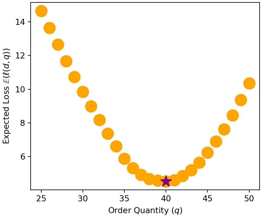
from numpy import linspace
import matplotlib.pyplot as plt
import pandas as pd

# initialize canvas and axes to plot on
## plot the results using matplotlib object-oriented interface
fig, ax = plt.subplots(figsize = [4.5,3.75], layout = "constrained");
ax.set_xlabel("Order Quantity" + r" ($q$)");
ax.set_ylabel("Expected Loss" + r" $\mathbb{E} \left(\ell(d,q)\right)$");

bestQ = 0
minLoss = float('inf')

for orderQty in range(25,50+1):
    expLoss = jnp.mean(lossGivenQ(q=orderQty))
    ax.scatter(orderQty,expLoss, s= 200, marker = "o", c = "orange");
    ## record to find minimum
    if expLoss < minLoss:
        minLoss = expLoss
        bestQ = orderQty

## place a purple star over the minimum
ax.scatter(bestQ,minLoss, s= 200, marker = "*", c = "purple");
plt.show();

Figure 3.10: Plotting expected loss to find the optimal order quantity of 40.

As opposed to trying every feasible order quantity, we can use gradient descent to get the same result. Let’s start our descent at $q=50$ to showcase taking steps in the negative direction.

# simulation parameters
stepSize = 1
maxSteps = 1000

# starting point
currentQ = 50. ## make float to avoid error

# expLossFunction
def expLossFun(q):
    expLoss = jnp.mean(lossGivenQ(q=q))
    return expLoss

# gradient of exp loss function
newsvGradient = grad(expLossFun)

# take steps towards optimum
for _ in range(0,maxSteps):
    gradientValue = newsvGradient(currentQ).item() #return just value
    ## break out of for loop is gradient val is sufficiently small
    if abs(gradientValue) < 0.1:
        break
    ## pick whether to increase or decrease order quantity
    ## NOTE: for minimizing steps are in direction of negative gradient
    if newsvGradient(currentQ) >= 0:
        ## if gradient is positive reduce q
        currentQ = currentQ - stepSize
    else:
        ## if gradient is negative increase q
        currentQ = currentQ + stepSize

# print optimum
print("The optimal order quantity is ", currentQ, " with expected loss of ", expLossFun(currentQ),".")

The optimal order quantity is  41.0  with expected loss of  4.5899997 .

Interestingly, our plot and gradient descent disagreed about the optimal order quantity $q^*$; our plotting exploration determined the optimal order quantity $q^* = 40$ and gradient descent determined $q^* = 41$. Figure 3.10 reveals why; the difference between expected loss with $q=40$ and $q=41$ is quite small. Since the difference is less than the 0.1 we used as our stopping rule (i.e. if abs(gradientValue) < 0.1: break), gradient descent stops at $q=41$ and never continues on to $q=40$.

3.6 Expected Utility Maximization Is Not Always Practical

Deviations between observed decision making under real-world uncertainty and behavior predicted by expected utility (EU) maximization are so frequently documented that EU (maximization) is only considered an approximation of a “good” or “rational” decision. Other decision quantification frameworks have emerged, like cumulative prospect theory or Choquet expected utility, but these frameworks often add to the burden of preference elicitation and, like expected utility, have mixed results in practice. Since humans are finicky and have very hard-to-pin down utility functions, we will downplay quantifying preferences using a single value when faced with decisions under uncertainty. Rather, when faced with uncertain outcomes, we will try to visually express how our actions lead to different outcome distributions. We will then ask decision makers to choose among visually presented outcome distributions that we, as analysts, deem most relevant. Eliciting preferences among infinite distributions is typically hard, but if we as analysts can present just relevant outcome possibilities, then maybe we have a shot at choosing a “good” decision.

3.7 Getting Help

As always, Google and YouTube should be your best friends. For a conceptual understanding of gradient descent, I recommend 3Blue1Brown’s video on gradient descent in neural networks at https://youtu.be/IHZwWFHWa-w. For gradient descent using jax, the jax documentation is probably the best resource out there at https://jax.readthedocs.io/en/latest/jax-101/01-jax-basics.html.

3.8 Questions to Learn From

Exercise 3.1 Categorize each of the below as defining an action, objective, or uncertainty:

The price you will pay for gasoline next week to fill up your car.
The price the gasoline station chooses to charge its customers for gasoline.
The purchase of a plane ticket for you to go on vacation.
The desire to go on vacation where it will be warm enough to swim.

Exercise 3.2 When creating a $100$-element representative sample of demand, properties of the sample will change with every simulation (assuming you have not fixed the seed). Go through the process of finding the min and max values of the 100-element array about twenty times. Which of the following best describes the typical min and max values that you see generating those twenty $100$-element sample of $X$ where $X \sim \textrm{Binomial}(200,0.2)$?

The minimum $X$ is always 27 and the maximum $X$ is always 50.
The minimum $X$ tends to be from 26-28 and the maximum $X$ tends to be from 48-52.
The minimum $X$ tends to be from 21-30 and the maximum $X$ tends to be from 49-62.
The minimum $X$ tends to be from 23-28 and the maximum $X$ tends to be from 52-58.
The minimum $X$ tends to be from 17-34 and the maximum $X$ tends to be from 41-74.
The minimum $X$ tends to be less than 25 and the maximum $X$ tends to be more than 65.
The minimum $X$ tends to be from 10-40 and the maximum $X$ tends to be from 30-70.
The minimum $X$ is usually 27 and the maximum is usually 50.
The minimum $X$ tends to be from 26-28 and the maximum $X$ tends to be from 48-52.
The minimum $X$ tends to be from 17-22 and the maximum $X$ tends to be from 60-65.

Exercise 3.3 When creating a $10,000$-element representative sample of demand, properties of the sample will change with every simulation (assuming you have not fixed the seed). Go through the process of finding the min and max values of the 10,000-element array about twenty times. Which of the following best describes the min and max values that are seen generating those twenty $10,000$-element samples of $X$ where $X \sim \textrm{Binomial}(200,0.2)$?

The minimum $X$ is always 27 and the maximum $X$ is always 50.
The minimum $X$ tends to be from 26-28 and the maximum $X$ tends to be from 48-52.
The minimum $X$ tends to be from 21-30 and the maximum $X$ tends to be from 49-62.
The minimum $X$ tends to be from 23-28 and the maximum $X$ tends to be from 52-58.
The minimum $X$ tends to be from 17-34 and the maximum $X$ tends to be from 41-74.
The minimum $X$ tends to be less than 25 and the maximum $X$ tends to be more than 65.
The minimum $X$ tends to be from 10-40 and the maximum $X$ tends to be from 30-70.
The minimum $X$ is usually 27 and the maximum is usually 50.
The minimum $X$ tends to be from 26-28 and the maximum $X$ tends to be from 48-52.
The minimum $X$ tends to be from 17-22 and the maximum $X$ tends to be from 60-65.

Exercise 3.4 The ticket manager at the Ryman Auditorium in Nashville, TN is contemplating how many VIP ticket packages (good seat + t-shirt are in the package) and how many general admission tickets (less good seat, but lower price) to offer for an upcoming John Prine tribute concert. If $Q$ represents the number of general admission tickets to offer for sale, $R^+$ represents the set of positive real numbers, and $Z^+$ represents the set of positive integers, which of the below sets might best represent the number of general admission tickets to offer up for sale. (you will probably need to look up the Ryman auditorium to get more context for this problem)

$Q \in \{q | q \in \mathbb{R}^+, 0 \leq q \leq 200\}$
$Q \in \{q | q \in \mathbb{Z}^+, 0 \leq q \leq 200\}$
$Q \in \{q | q \in \mathbb{R}^+, 0 \leq q \leq 2,000\}$
$Q \in \{q | q \in \mathbb{Z}^+, 0 \leq q \leq 2,000\}$
$Q \in \{q | q \in \mathbb{R}^+, 0 \leq q \leq 20,000\}$
$Q \in \{q | q \in \mathbb{Z}^+, 0 \leq q \leq 20,000\}$
$Q \in \{q | q \in \mathbb{R}^+, 0 \leq q \leq 100\}$
$Q \in \{q | q \in \mathbb{Z}^+, 0 \leq q \leq 100\}$
$Q \in \{q | q \in \mathbb{R}^+, 0 \leq q \leq 3,000\}$
$Q \in \{q | q \in \mathbb{Z}^+, 0 \leq q \leq 3,000\}$
$Q \in \{q | q \in \mathbb{R}^+, 0 \leq q \leq 40,000\}$
$Q \in \{q | q \in \mathbb{Z}^+, 0 \leq q \leq 40,000\}$
$Q \in \{q | q \in \mathbb{R}^+, 0 \leq q \leq 50\}$
$Q \in \{q | q \in \mathbb{Z}^+, 0 \leq q \leq 50\}$
$Q \in \{q | q \in \mathbb{R}^+, 0 \leq q \leq 4,000\}$
$Q \in \{q | q \in \mathbb{Z}^+, 0 \leq q \leq 4,000\}$
$Q \in \{q | q \in \mathbb{R}^+, 0 \leq q \leq 50,000\}$
$Q \in \{q | q \in \mathbb{Z}^+, 0 \leq q \leq 50,000\}$

Exercise 3.5 Match each company to the performance metric (i.e. outcome of interest) best-associated with that company. Read about company strategies on the Internet as needed. Each company and each outcome should be used only once.

Company	Draw line from Company to Outcome of Interest	Outcome of Interest
Costco		Total Unsubscribes
Zapier		Product Margin
Lendable		Financed Solar Homes
Tesla		Accidents Per Mile
MailChimp		Total Number of Integrated Apps

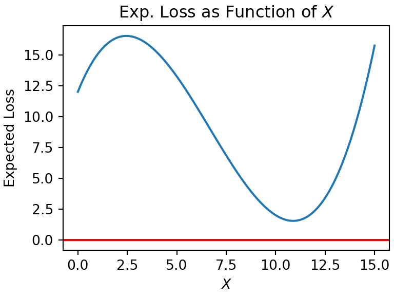
Exercise 3.6 Given the plot in Figure 3.11. What is the optimal action?

Figure 3.11: Expected loss as a function of X.

$X$ should be around 0.
$X$ should be around 2.5.
$X$ should be around 11.
$X$ should be around 15.
Expected loss should be very close to 0.
Expected loss should be around 2.5.
Expected loss should be around 11.
Expected loss should be around 15.

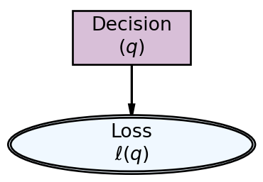
Exercise 3.7

Figure 3.12: Graphical model for a decision.

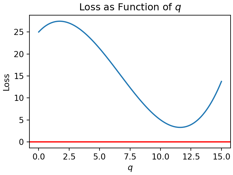
Let’s examine optimizing the decision pictured in Figure 3.12 where $Q \in \{q|q \in \mathbb{R}, 0 \leq q \leq 15\}$ and the decision-maker (DM) is minimizing loss as a function of $q$. For this DM, plotting loss $\ell(q)$ versus decision $q$ yields the graph in Figure 3.13.

Figure 3.13: Expected loss as a function of q.

No math or coding is required. Use Figure 3.13 to mark all of the following statements regarding this decision problem as TRUE or FALSE:

( T / F ) The gradient at $q=0.5$ is positive and using gradient descent would lead to choosing a smaller $q$ for the next iteration.
( T / F ) The gradient at $q=7.5$ is positive and using gradient descent would lead to choosing a smaller $q$ for the next iteration.
( T / F ) The gradient at $q=14$ is positive and using gradient descent would lead to choosing a smaller $q$ for the next iteration.
( T / F ) There are two values of $q$ for which the gradient is zero.
( T / F ) Starting gradient descent at $q = 5.0$ and starting gradient descent at $q = 14$ will likely lead to more similar optimal solutions when compared to the difference in optimal solutions of starting gradient descent at $q = 1.0$ and starting gradient descent at $q = 3.5$.
( T / F ) The optimal decision is $q=7.5$.
( T / F ) The optimal decision $q$ is greater than 7.5.
( T / F ) The optimal decision $q$ is less than 7.5.

Exercise 3.8 Let’s examine optimizing the decision pictured in Figure 3.12 where $Q \in \{q|q \in \mathbb{R}, 0 \leq q \leq 15\}$ and assuming loss can be expressed as the following function of decision $q$:

\[ \ell(q) = 3q - q^2 + \tfrac{q^3}{20} + 25 \]

Create code to perform a gradient descent optimization of $q$. Use $q=5$ as your initial value (hint: code this value as a float, not an int), a step-size of $\gamma = 0.0125$, and a stopping criteria of either a maximum of 600 steps or the magnitude of the gradient (i.e. absolute value) at the current $q$ is less than 0.1.

What value do you get for the optimal $q$? (students should upload code to verify that gradient descent was used)

Exercise 3.9 WARNING: the seed value will change on each attempt.

Returning to our newsvendor example, the graphical model of Figure 3.14 shows the explicit dependence of our objective function on our uncertainty about demand and our decision on how much to order.

Figure 3.14: Graphical model of the newsvendor’s decision model.

The statistical model accompanying Figure 3.9 is shown here:

\[ \begin{aligned} D &\equiv \textrm{Daily demand for newspapers, and}\\ D &\sim \textrm{Binomial}(n=200,p=0.2).\\ Q &\equiv \textrm{Order quantity chosen by decision-maker, where}\\ Q &\in \{0, 1, 2, \ldots, 200\}.\\ \pi &\equiv \textrm{Quantification of the newsvendor's profit.}\\ \pi(d,q) &= 3.50 * \min(d,q) - q . \end{aligned} \]

Above, the newsvendor model is reframed as a profit maximization problem where each newspaper costs $1 and is sold for $3.50 to customers. Use the below code for your profit function and for getting a representative sample of demand:

WARNING: the seed value in the below code will change on each attempt.

# !pip install matplotlib --upgrade  ##uncomment for Colab
import pandas as pd
from jax import grad
import jax.numpy as jnp
from numpy.random import default_rng
from functools import partial

## write profit function in Python
def profitFunction(d,q):
    revenue = jnp.minimum(d,q) * 3.50
    expense = q   
    profit = revenue - expense
    return profit

potentialCusts = 200
purchaseProb = 0.2

rng = default_rng(seed = 111) ##THIS VALUE CHANGES WITH EACH ATTEMPT
numSims = 100

# create data frame to store simulated demand
newsDF = pd.DataFrame({"simNum": range(1, numSims+1),  # sequence of 1 to 100
                   "demand": rng.binomial(n = potentialCusts, 
                                          p = purchaseProb,
                                          size = numSims)})

## convert from pandas series type to jax array
## all input arrays should be jax arrays for optimizing
demand = jnp.array(newsDF.demand)

Add to the above code to use gradient ascent to find the optimal order quantity for maximizing expected profit. Use the 100-element representative sample of demand to simulate expected profit as a function of order quantity, start at $q=50.0$, use a step size of $\gamma = 1.0$, and a maximum number of steps as 100. The stopping criteria should be when the magnitude of the gradient at the current step’s order quantity is less than 0.1.

What value do you get for the expected profit at the optimal $q$ (round to the nearest penny)? (students should upload code to verify that gradient descent was used)

WARNING: the seed value will change on each attempt.

Exercise 3.10 ( True or False ) Expected utility maximization is the greatest intellectual construct of our time and we will rely on it almost exclusively in this textbook.