In this chapter, we explore the xarray package; Python’s premiere package for dealing with labelled multi-dimensional arrays. Let’s digest what that means. Labelled simply means we can use English names instead of numbers to identify data elements; it is so much more intuitive to ask the computer to “give the expected profit associated with decision q” than it is to ask something like “give the element of the axis” as would be done if using numpy. You might balk and say pandas can have names for rows and columns, and that is true, but what if you need to reference data which requires more than two coordinates as, say, specified by a row and a column in pandas. For example, storing weather related data requires dimensions of “latitude”, “longitude”, and “time” and for each combination of those three dimensions one might want access to multiple data variables like “temperature”, “precipitation”, and “wind speed”. Trying to put that data inside of pandas would be cumbersome and putting that data into numpy would certainly be less intuitive than using nice English labels like “precipitation”. So, labelled multi-dimensional means that data elements can be indexed by as many labels as makes sense and xarray makes this beautifully elegant.
In this chapter, we will start exploring the xarray package by increasing the complexity of our study of the newsvendor problem. Let’s start our journey with Example 5.1.
Example 5.1 We again revisit a newsvendor with a single opportunity to buy newspapers in the morning and then to sell those newspapers on a city corner throughout the day. Our newsvendor’s objective is expressed in two outcomes of interest, namely profit and lost sales, for which he seeks a good combo of high profit and low levels of lost sales; customers who do not find the newspaper are more likely to switch to a different newsvendor. Newspapers are purchased for $1 and sold for $3. Papers remaining at the end of the day are worthless. The newsvendor faces demand that is binomially distributed with parameters and . Let’s help the newsvendor make a good decision by effectively visualizing possible decisions and the associated outcome distributions for profit and service level.
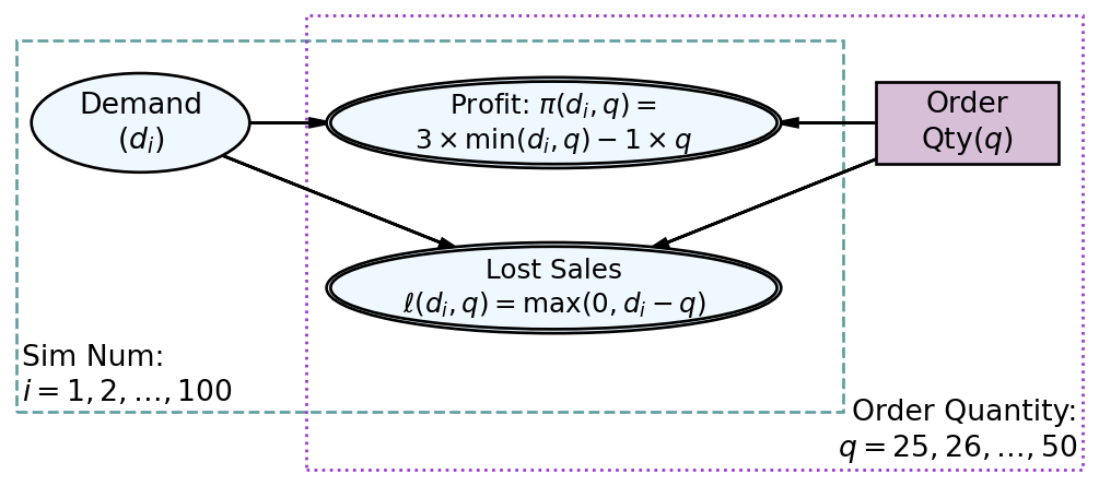
The graphical model of Figure 5.1 shows the explicit dependence of our two outcomes of interest on uncertainty about demand and our decision on how much to order.
Figure 5.1: The newsvendor has two outcomes of interest, profit and lost sales.
Around the nodes, notice the new addition of rectangles,technically called plates. When we see any node presented in a graphical model, we should be thinking of a single realization of that random variable. Inclusion of nodes within a plate represents the fact that our model replicates those nodes once per index of the plate. In Figure 5.1 for example, demand has one realization per each of the 100 simulations; is the demand of the simulation and thus, would be the random demand of the simulation. The statistical model accompanying Figure 5.1 is shown here:
To put the graphical model into code, we previously used a dataframe to store a representative sample of demand and the associated outcomes of interest for a decision. We can repeat that here for just one order quantity, say :
potentialCusts =200purchaseProb =0.2rng = default_rng(seed =111) numSims =100# create data frame to store simulated demandnewsDF = pd.DataFrame({"simNum": range(1, numSims+1), # sequence of 1 to 100"demand": rng.binomial(n = potentialCusts, p = purchaseProb, size = numSims)})## google SEARCH PHRASE: get element-wise minimum of two columns in pandas dataframenewsDF["profit_q42"] =3* np.minimum(newsDF.demand,42) -1*42newsDF["lostSales_q42"] = np.maximum(0,newsDF.demand -42)# view first few 5 rows of newsDFnewsDF.iloc[:5,:]
But now, imagine we want to consider all integer order quantities ranging from 25 to 50; that is 26 different order quantities. It will feel cumbersome to add 52 columns, one for each order quantity’s profit and one for each quantity’s lost sales, into a dataframe. There must be a better way to structure how we store this data. More naturally, we can imagine having 26 dataframes, each one specific to a particular order quantity. However, the problem there is we either repeat the simNum and demand columns for each of the 52 data frames, or we omit those columns from the 52 dataframes and somehow know the correspondence of rows in the profit/loss dataframes to rows in the simNum/demand dataframe. All of this just does not feel right, we are repeating data or hiding knowledge about the data’s structure. The answer for us is in a package called xarray that specializes in handling this type of multi-dimensional labelled data problem.
5.1 The xarray Package
Our goal is to elegantly match our data storage structure to the dimensions of the problem and to increase our ability to work with lots of data using human-interpretable labels. We will do that using the two main data structures from the xarray package.
It might take your brain a little extra work to use this package, but in the end you will be more resilient for it; embrace a little productive struggle here, its worth it.
The first structure is a DataArray. In its simplest 1-dimensional form, a DataArray is just a collection of values, like the column of dataframe (pandas.Series) or a one-dimensional array of values (numpy.ndarray). We can create a simple DataArray using its constructor function. The DataArray created here is a container for a 100-element representative sample of demand corresponding to the narrative of Example 5.1:
from numpy.random import default_rngimport numpy as npimport xarray as xrrng = default_rng(seed =111) ## set random seed demand = rng.binomial(n=200,p=0.2,size=100) ## get demand values## make data arrayxr.DataArray(data = demand)
Above, we see a 100-element array containing our simulated demand values, but we also see some other things, notably a dim_0: 100 and placeholders for coordinates and attributes. Let’s tackle these one-by-one. First, the dimension key-value pair dim_0: 100 tells us that the cardinality of our demand array is 100 (i.e. there are 100 values) and the name of the index or coordinate-axis is dim_0. In numpy, axes are indexed using numbers like etc., but when using xarray we will always want to give our indexes more meaningful and human-interpretable names. When it comes to drawing random samples, we logically name the demand array’s dimension as draw and implement this in code using the dims argument:
## make data array with labelled dimension namexr.DataArray(data = demand, dims ="draw")
where the output now replaces dim_0: 100 with draw: 100 telling us there are 100 draws of demand. It will come in handy for us to be able to refer to specific draws, say draw #3, so we label these draws. Every label value used for indexing an array is called a coordinate. We add the coordinates to our array of demand using a dict-like object supplied to the coords argument:
The one argument numpy.arange(stop) function returns an array of integers starting at 0 and ending at stop - 1. Mathematically, it returns an array of integers on the half-open interval [0, stop). Thus, numpy.arange(100)+1 gives us a set of 100 integers starting at 1 and ending at 100 (inclusive).
## explicit labeling of coordinates - must use name now to create dataset laterdemandDA = xr.DataArray(data = demand, coords = {"draw": np.arange(100)+1}, name ="demand")demandDA
Notice, we can drop the dims arguments as the dimension name is supplied in the dictionary object passed to the coords argument.
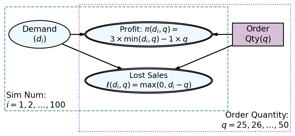
Figure 5.2: The newsvendor has two outcomes of interest, profit and lost sales.
Recall the graphical model of Figure 5.1, reproduced here in the margin as Figure 5.2 for convenience. We have started a mapping of graphical model elements to code equivalents in the xarray package. We have an array of demand values, , indexed by . The values are the values of the DataArray and the index is the coordinates; is the label we use to refer to the draw number of each demand value. Analogously, order quantity, , can be thought of as the label we use to refer to each order quantity - somewhat confusingly though the array value for order quantity and the label we use to refer to that order quantity are the same. In general, plate indices will map to coordinates and decision/random variable nodes will map to data arrays. Following this rule, let’s make a new data array for order quantity where index and array value get identical quantities - the index represents the order-quantity plate index in Figure 5.1 and the data is mapped from the rectangular decision node.
## creating a DataArray of order quantities - must use name now to create dataset laterorderDA = xr.DataArray(data = np.arange(25,51), coords = {"orderQtyIndex": np.arange(25,51)}, name ="orderQty")orderDA
Now for the magic! We will create the second data structure of the xarray package, the Dataset. A Dataset is a container for related DataArray objects. As Figure 5.2 shows, we need both demand and order quantity to calculate our outcomes of interest, namely profit and lost sales. We will soon see that placing demand and order quantity in the same Dataset allows us to easily derive the DataArray objects for profit and lost sales; both of which are indexed by and as they are contained in both the Sim Num and Order Quantity plates.
Creating a Dataset from existing DataArray objects is accomplished by passing a list of data array(s) to the merge function which will return a dataset:
# create dataset by combining data arraysnewsvDS = xr.merge([demandDA,orderDA])newsvDS
The cardinality of a set is the number of elements in the set. Symbolically, the absolute value notation, is used to express cardinality of a set. The Cartesian product of two sets and , denoted , is the set of all combinations (ordered pairs) with one element from and one-element from . The cardinality of the Cartesian product is the product of the cardinalities of the input sets, i.e. . See this wikipedia entry on Cartesian products for more info.
Our Dataset container now has the dimensions implied by the plate indices in Figure 5.1, namely draw: 100 orderQty: 26. In math terms we have two sets, one is a set of demand draws where cardinality ; the other a set of order quantities with cardinality . Thus, the set of all ordered pairs to be used for calculation of profit and lost sales will have cardinality . Thus, our simulation of potential and values will each have 2,600 elements.
5.2 Seven mental models of dataset manipulation
To calculate the 2,600-elements we will use the first of seven categories of important data manipulations known as the seven mental models of dataset manipulation (inspired by Wickham et al. (2022)). We quickly list the seven mental models here before continuing on towards our objective of how to calculate representative samples of profit and lost sales for each potential order quantity.
Wickham, Hadley, Romain François, Lionel Henry, and Kirill Müller. 2022. Dplyr: A Grammar of Data Manipulation.
“Seven mental models of dataset manipulation” is not an industry standard term. Its a mnemonic device for us to recognize that seven functions will get you most of what you need for manipulating datasets. I take inspiration from Hadley Wickham’s verbs of data manipulation which have been wildly successful in simplifying the ease with which one’s brain is translated into data manipulating code.
The seven most important ways we might want to manipulate a data array or dataset is to:
Assign: .assign() or assign_coords(): Add data variables with broadcasting and array math. (Can also use dict-like methods)
Subset: .sel() or .where() subset a data array or dataset based on coordinates or data values, respectively.
Drop: .drop_vars() or .drop_dims(): Remove an explicit list of data variables or remove all data variables indexed by a particular dimension.
Sort: .sortby() sorts or arranges a data array or dataset based on data values or coordinate values.
Aggregate: See the xarray documentation for a list of aggregation functions. These functions will collapse all the data of a given dimension; for example one can collapse a time dimension using the mean() aggregation method to get the average value for all of time.
Split-Apply-Combine: .groupby() and DatasetGroupBy.foo() are usually used in combination to 1) split the dataset into groups based on levels of a variable, 2) apply a function (e.g. foo()) to each group’s dataset individually, and then 3) combine the modified datasets. See the xarray documentation for more details.
Merge(join): Getting information from two datasets to intelligently combine.
5.2.1 Assign: Adding Data Arrays
Recapping what has been done from a graphical model perspective, we created DataArray objects for all of the nodes that lack parent nodes in the graphical model, like and in Figure 5.2, and then we used merge() to create a dataset containing all the parentless data arrays, as they are the basis for our coordinates and all additional computations. Now, introduced here, we use the .assign() method to create new data variables for all the other (children) nodes of the graphical model.
Notice the term used in calculating profit. This term actually represents the number of newspapers sold for any ordered pair of . If demand exceeds the order amount, then the newsvendor can still only sell newspapers. And if the newsvendor over-orders, , then the newsvendor can only sell newspapers.
( ## open parenthesis to start readable code newsvDS .assign(soldNewspapers = np.minimum(newsvDS.demand,newsvDS.orderQty))) ## close parenthesis finishes the "method chaining"
( ## open parenthesis to start readable code newsvDS .assign(soldNewspapers = np.minimum(newsvDS.demand,newsvDS.orderQty)) .assign(revenue =3* newsvDS.soldNewspapers)) ## close parenthesis finishes the "method chaining"
The above code will yield an error:
AttributeError: 'Dataset' object has no attribute 'soldNewspapers'
The last assignment apparently does not have visibility into the newly created data for soldNewspapers. To pass the current state of the dataset to the .assign() method, we use a lambda function. The lambda function has syntax lambda arguments : expression where lambda is a keyword telling python to expect an argument (or arguments), followed by a colon (:), and then an expression for what will be returned by the function; in our case here, the argument will provide a way of referencing the current state of the dataset in the method chain. We will call it DS to signal to our brain that the .assign() method is receving a dataset. Here is updated code that works:
( ## open parenthesis to start readable code newsvDS .assign(soldNewspapers = np.minimum(newsvDS.demand,newsvDS.orderQty)) .assign(revenue =lambda DS: 3* DS.soldNewspapers)) ## use lambda function to get current state of dataset in chain
Yes, I think the need to use lambda functions creates unnecessary cognitive friction. I wish it was easier. That being said, method chaining creates such readable and debuggable code, it is worth incurring a little overhead now to learn about lambda functions.
Now, along with some intermediate variables to enhance understanding of the math, we create the two primary outcomes of interest which are profit and lost sales. We also convert all assignments into lambda functions so that we may use this method chain with another dataset. Lastly, a two-line combo converts our dataset to a dataframe so that we may take an error-checking peek at few observations of our outcomes:
newsvDS = (newsvDS .assign(soldNewspapers = np.minimum(newsvDS.demand,newsvDS.orderQty)) .assign(revenue =lambda DS: 3* DS.soldNewspapers) .assign(expense =1* newsvDS.orderQty) .assign(profit =lambda DS: DS.revenue - DS.expense) .assign(lostSales = np.maximum(0, newsvDS.demand - newsvDS.orderQty)))(newsvDS .to_dataframe() #dataframe for printing .sample(5, random_state =111)) ## show five rows of DF
Note, one can also add columns directly using dict-like indexing when chains of operations are not required. The following code would work similarly to what we did earlier:
5.2.2 Select a subset of the data array or dataset
Recall the syntax of help documentation is often packagename.Class.method where class is typically capitalized. So, when referring to a method like sel() that is available for Dataset object in the xarray package, documentation will refer to the method as xarray.Dataset.sel. Sometimes for brevity, I will drop that package name and use Dataset.sel. Also recall that to use a method, add parentheses after the method name, i.e. sel().
To reduce a dataset or data array by selecting a subset of coordinates to keep, use the associated methods: Dataset.sel() or DataArray.sel.
# select a particular value for a dimensionnewsvDS.sel(orderQtyIndex =36) # returns 1-d dataset
xarray follows the pandas convention for selecting a range of coordinate values to keep using the slice function.
# slicing returns all values inside the range (inclusive)# as long as the index labels are monotonic increasingnewsvDS.sel(orderQtyIndex =slice(36,38))
Slicing returns a smaller dataset or data array based on coordinates, but often we want a smaller dataset based on data values. In these cases, we apply the .where() method where the argument is some logical condition for which data to keep:
# need to explicitly use DataSet.DataArray syntax for# filtering out rows that do not meet conditionnewsvDS.where(newsvDS.lostSales >0)
<xarray.Dataset>
Dimensions:         (draw: 100, orderQtyIndex: 26)
Coordinates:
  * draw            (draw) int32 1 2 3 4 5 6 7 8 9 ... 93 94 95 96 97 98 99 100
  * orderQtyIndex   (orderQtyIndex) int32 25 26 27 28 29 30 ... 46 47 48 49 50
Data variables:
    demand          (draw, orderQtyIndex) float64 42.0 42.0 42.0 ... nan nan nan
    orderQty        (orderQtyIndex, draw) float64 25.0 25.0 25.0 ... nan nan nan
    soldNewspapers  (draw, orderQtyIndex) float64 25.0 26.0 27.0 ... nan nan nan
    revenue         (draw, orderQtyIndex) float64 75.0 78.0 81.0 ... nan nan nan
    expense         (orderQtyIndex, draw) float64 25.0 25.0 25.0 ... nan nan nan
    profit          (draw, orderQtyIndex) float64 50.0 52.0 54.0 ... nan nan nan
    lostSales       (draw, orderQtyIndex) float64 17.0 16.0 15.0 ... nan nan nan
Often times, the lambda syntax for anonymous functions gets used to pass in the dataset name:
(newsvDS.where(lambda x: x.lostSales >0, drop =True) .to_dataframe() #convert to pandas dataframe for printing .dropna() # pandas method to remove NaN rows .sample(5, random_state =111))
You should experiment with omitting the pandas.DataFrame.dropna method from the above. Because filtering on data variables does not change the coordinate system, many coordinate combinations that are of part of the xarray dataset will have missing values because the values that were there did not survive the filtering process (e.g. lostSales > 0).
For more information on selecting subsets of datasets or arrays, or dropping a data array from an existing dataset, this xarray tutorial on selecting and indexing data is useful https://docs.xarray.dev/en/stable/user-guide/indexing.html.
5.2.3 Drop Dimensions
The drop_dims() method returns a new object by dropping a full dimension from a dataset along with any variables whose coordinates rely on that dimension.
Above, the order quantity dimension is dropped along with all the data variables whose value depended on order quantity: orderQty, soldNewspapers, revenue, expense, profit, and lostSales.
If you want to just drop some of the data variables, you use drop_vars():
5.2.4 Sort a data array or dataset based on data values or data values.
For us, sorting is best done outside of xarray. We will typically want dataframe-like reports generated out of xarray as a last step in data manipulation. We will rely on pandas.DataFrame.sort_values() to help us for this mental model.
This is the mental model we will use to report summary statistics (mean, median, quantile); we will use it throughout the remainder of this textbook.
We have a two-step process:
Aggregate the information in a data array.
Assign the output of the aggregation to a new data array in a pre-existing dataset.
By way of example, let’s get the expected profit associated with each order quantity for our newsvendor in Example 5.1. Currently, our dataset, newsvDS, has 100 values (one for each draw) for each of the 26 order quantities. What we want is just 1-value for each of the 26 order quantities; so, we seek to collapse all 100 draws for an order quantity into 1 number representing the mean profit. Starting this process, we aggregate the profit array along the dimension(s) we want to collapse, in this case we no longer want the draw dimension:
## collapse the 100 draws into 1 summary statisticnewsvDS.profit.mean(dim ="draw")
Notice, this returns a DataArray object. We will then keep our data and summary statistics together in one dataset by adding the array back to the original dataset using assign(). Here the two-step workflow is demonstrated to return expected profit and expected lost sales for each order quantity:
Under “Data Variables” notice expProfit and expLoss are one-dimensional with that one-dimension being orderQtyIndex. Pretty cool how we can compactly store all this related information in one dataset! Feel free to play around with these other frequently-used aggregation functions include count, first, last, max, mean, median, min, quantile, and sum.
5.2.6 Split-Apply-Combine
.groupby() and DatasetGroupBy.foo() are usually used in combination to 1) split the dataset into groups based on levels of a variable, 2) apply a function (e.g. foo()) to each group’s dataset individually, and then 3) combine the modified datasets. See the xarray documentation for more details. Here is a small sample fo code:
## find average profit by orderQty## see documentation here: https://docs.xarray.dev/en/stable/generated/xarray.core.groupby.DatasetGroupBy.mean.html( newsvDS .get("profit") .groupby("orderQtyIndex") .mean(...)).to_dataframe()
Here, we can bring in information from another dataset. More info for this section is forthcoming.
5.3 Getting Help
The best place to learn about xarray is its help documentation available at https://docs.xarray.dev/en/stable/index.html. Additionally, YouTube has some tutorials available if you search there.