6 Plausibility, The Beta Distribution, and Its Visualization
“She was blocked because she was trying to repeat, in her writing, things she had already heard, just as on the first day he had tried to repeat things he had already decided to say. She couldn’t think of anything to write about Bozeman because she couldn’t recall anything she had heard worth repeating. She was strangely unaware that she could look and see freshly for herself, as she wrote, without primary regard for what had been said before. The narrowing down to one brick destroyed the blockage because it was so obvious she had to do some original and direct seeing.” - Zen and The Art Of Motorcycle Maintenance
In this chapter, I will try to empower you with the ability to allocate your plausibility over sample spaces. Recall, a sample space is just a set of all possible outcomes; so, your empowerment will be the ability to allocate plausibility, a total of 100% probability, to any set of outcomes that interest you.
Lets’ start simple and consider these two possible outcomes:
- The sun will explode tomorrow.
- The sun will not explode tomorrow.
Ahh yes, a Bernoulli random variable. Let’s get rigorous and add the graphical and statistical models defining this sample space:
\[ \begin{aligned} X &\equiv \textrm{RV for sun explosion. Sun explosion}=1 \textrm{ and no explosion}=0.\\ X &\sim \textrm{Bernoulli}(p=100\%) \end{aligned} \]
Now, imagine I ask you to create a representative sample of \(X\) using 5 elements in the sample; thus, each sample draw would represent 20% plausibility. I am pretty confident that you and others would all use this representative sample:
import xarray as xr
sunExplodes = xr.DataArray([0,0,0,0,0])
While you and I, being cool data analysts, could comprehend that a representative sample of all zeroes means the sun will NOT explode tomorrow, its often helpful to visualize this allocation of plausibility. I show two ways here.
ArviZ is a Python package used for exploratory analysis of Bayesian models (which we will learn more about soon). For now, think of it as a plotting package, compatible with matplotlib, that we use for displaying representative samples.
import matplotlib.pyplot as plt
import numpy as np
import arviz as az
plt.style.use("seaborn-whitegrid")

## plot the results using matplotlib object-oriented interface
fig, axs = plt.subplots(ncols = 2,
                        figsize=(10, 3.5),
                        layout='constrained')
fig.suptitle("The Sun Will Not Explode Tomorrow", fontweight = "bold")

# dot plot construction
az.plot_dot(sunExplodes, ax = axs[0])
axs[0].set_title("A Dot Plot - Each Dot Allocates 20% Plausibility")
axs[0].set_xlim(-0.25,1.25)
axs[0].set_xticks([0,1], labels = ["No Explosion", "Explosion"])
axs[0].set_ylabel("Plausibility")

# histogram construction
az.plot_dist(sunExplodes, ax = axs[1])
axs[1].set_title("A Distribution Histogram - Height of the Bar is Plausibility")
axs[1].set_xlim(-1,2)
axs[1].set_xticks([0,1], labels = ["No Explosion", "Explosion"])
axs[0].set_ylabel("Plausibility")

plt.show()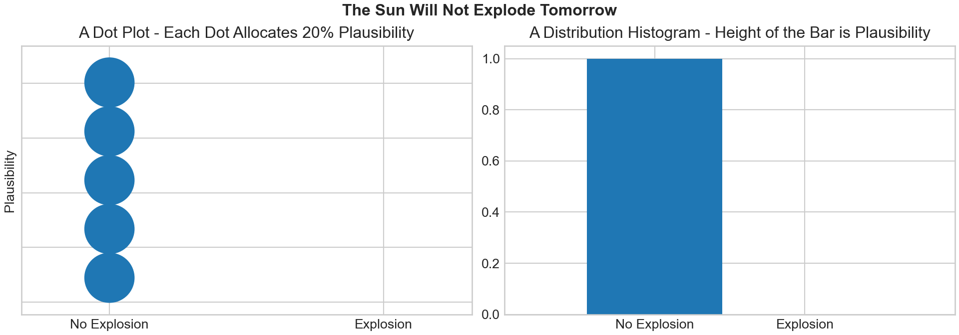
Figure 6.2 (right) is directly interpretable. The x-axis gives the two outcomes and y-axis is the plausibility measure. When outcomes are discrete, the height of the plausibility measure is directly interpretable as a probability. We can see that the height of “No Explosion” is 1, meaning we assign 100% probability to the sun not exploding. In math notation,
\[ P(X=0) = f_X(0) = 1 = 100\%. \] Figure 6.2 (left), known as a quantile dotplot (https://github.com/mjskay/when-ish-is-my-bus/blob/master/quantile-dotplots.md), is also directly interpretable. In this case, each dot represents 20% plausibility (because there are 5 dots and plausibility should sum to 100%). Counting dots gives a probability estimate.
6.1 The Uniform Distribution
Now, let’s imagine a case where there are infinite outcomes, not just two or some other countable number of outcomes. For example, there are infinitely many real numbers between 0 and 1, such as 0.123456789876543 or 0.987654323567. If we want to allocate 100% plausibility to those infinite outcomes, how might we do it? The answer is to use a continuous probability distribution.
Unlike a discrete probability distribution, where probability mass function \(f_X(x)\) denoted the probability of a random variable equaling \(x\), i.e. \(P(X=x)\), in the continuous world, \(x\) can take on infinite values and its probability density function \(f_X(x)\) represents a notion of plausibility, but not a probability; all we can say is the higher plausibility measure \(f_X(x)\) is, the more likely \(x\) is. But we also would say \(P(X=x)=0\) because the chances of getting any one particular \(x\)-value can be thought of as:
\[ P(X=x)=\frac{1}{\infty} \approx 0. \] Let’s take an example of a standard uniform distribution whose support is \((0,1)\) and all of the infinite values between 0 and 1 are equally likely. In this case, visualize spreading probability over a two-dimensional shape where the area of the shape is restricted to be one or 100%. One dimension of the shape is the x-axis and it is determined by the support, i.e. 0 to 1. And, the other dimension will be the height above the x-axis, the y-axis coordinate, which happens to be specified by the probability density function \(f_X(x)\), which we are declaring to be our plausbility measure. Let’s see this visually in Figure 6.3.
# !pip install arviz matplotlib --upgrade

import scipy.stats as stats
import numpy as np
plt.style.use("seaborn-whitegrid")

x = stats.uniform()

# generate evenly spaced points from the support
supportOfX = np.linspace(0,1, num = 100)

# calculate  the probability density function at each point from support
pdfOfX = x.pdf(supportOfX)

## plot uniform pdf
fig, ax = plt.subplots(figsize=(6, 3.5), layout='constrained')
ax.fill_between(supportOfX, pdfOfX,color = 'aliceblue')
ax.plot(supportOfX, pdfOfX,
       color = 'cadetblue', lw=5,  label='uniform pdf')
ax.annotate(text = "Area under blue line is 100%\n Width = 1 and Height = 1",
            xy = (0.5,0.5), xytext = (0.5,0.5),
            horizontalalignment='center', fontsize = 18)
ax.set_title("Plausibility is Evenly Distributed To All Numbers Between Zero and One")
ax.set_ylim(0,1.2)
ax.set_ylabel('Plausibility Measure: ' + r'$f_X(x)$')
ax.set_xlabel(r'$x$')

plt.show()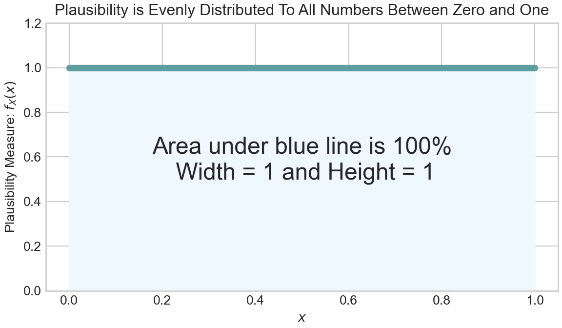
In Figure 6.3, notice the height of the density function \(f_X(x) = 1\) for \(0 \leq x \leq 1\). Also notice the width of the shaded area is determined by the support of \(x\), so the width is 1. So if area is equivalent to probability, we can calculate the area of the shaded rectangle in Figure 6.3 as width \(\times\) height to confirm that indeed the area is 1 or 100%. So, we can say \(P(0 \leq X \leq 1) = 100\%\). Let’s make another probabilistic statement using area to represent probability. For example, if
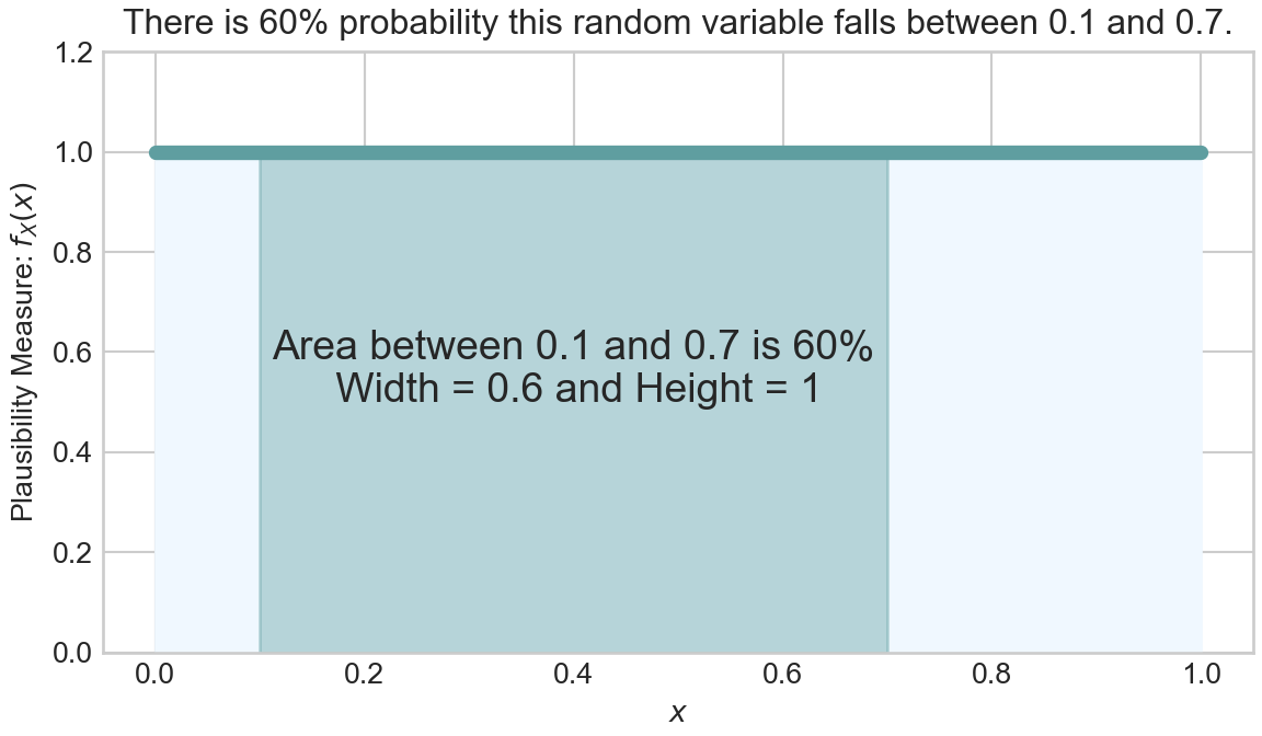
\[ X \sim \textrm{Uniform}(0,1) \] then, we can calculate the probability that \(X\) is between 0.1 and 0.7 by looking at the area under the density function as shown in Figure 6.4.
Thus, we can make the probabilistic statement that \(P(0,1 \leq X \leq 0.7) = 100\%\)
In a continuous world, before having helpful computers, we would use calculus to calculate the area (note: you will not be doing any derivatives by hand in this book’s exercises). From calculus, the following must hold for any valid probability density function, \(f_X(x)\):
\[ \int_{-\infty}^{\infty}f_X(x)dx = 1 \] which simply means the area under the probability density function must be one. For illustration purposes only, we show how calculus would find that \(P(0.1 \leq x \leq 0.7) = 60\%\). First, from Wikipedia we find for a uniformly distributed random variable:
\[ f_X(x) \equiv \begin{cases} 1, & \textrm{if } 0 \leq x \leq 1 \\ 0, & \textrm{otherwise} \end{cases} \] Hence, the area under the density function from 0.1 to 0.7 is
\[ \int_{0.1}^{0.7}f_X(x)dx = \int_{0.1}^{0.7} 1 \textrm{ } dx = \left[x\right]_{0.1}^{0.7} = 0.7 - 0.1 = 0.6 = 60\% \]
which is exactly the number we get doing simple width \(\times\) height in Figure 6.4. For our purposes, let’s just takeaway the intuition that it is the area under the density curve which represents probability in a continuous probability distribution. In the next section, we explore a distribution with support of \((0,1)\), but for which plausibility does not have to be spread evenly.
6.2 The Beta Distribution
A \(\textrm{beta}\) distribution is a two-parameter distribution whose support, just like the standard uniform distribution, is \([0, 1]\). The two-parameters are typically called \(\alpha\) (alpha) and \(\beta\) (beta); yes, it is annoying and might feel confusing that the \(\textrm{beta}\) distribution has a parameter of the same-name, \(\beta\), but generally, it is clear from context which one you are talking about. Let’s assume random variable \(\Theta\) (capital “theta”) follows a \(\textrm{beta}\) distribution. Hence,
\[ \Theta \sim \textrm{beta}(\alpha,\beta) \]
Just like with any random variable, if we can create a representative sample, then we can understand which values are likely and which are not. In Python, we will continue to create representative samples using numpy’s random number generation methods. The syntax is default_rng().beta(a,b,size) where size is the number of draws, a is the argument for the \(\alpha\) parameter, and b is the argument for the \(\beta\) parameter. Hence, if we assume
\[ \Theta \sim \textrm{beta}(6,2) \]
then we can plot a representative sample:
from numpy.random import default_rng
from numpy import linspace
import arviz as az
rng = default_rng(seed = 111)
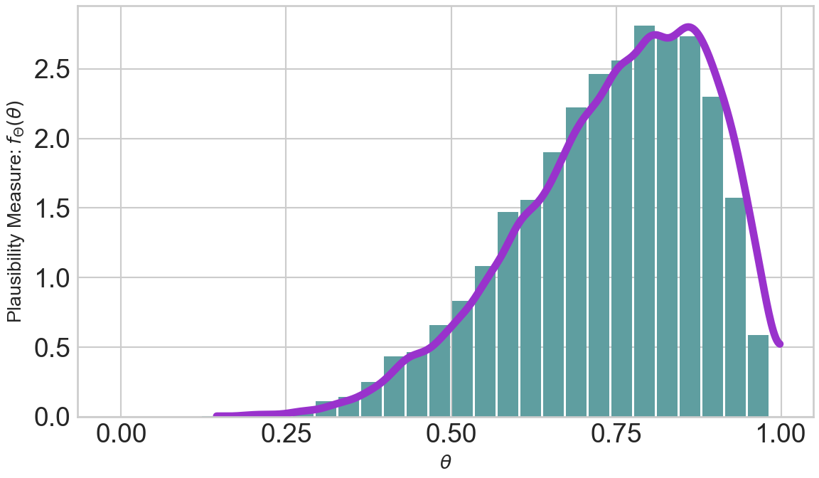
repSampBeta6_2 = rng.beta(a = 6, b = 2, size = 10000)
fig, ax = plt.subplots(figsize=(6, 3.5),
layout='constrained')
# plot histogram
az.plot_dist(repSampBeta6_2, kind = "hist", color = "cadetblue", ax = ax,
hist_kwargs = {"bins": linspace(0,1,30), "density": True})
# plot density estimate, i.e. estimate of f(x)
az.plot_dist(repSampBeta6_2, ax = ax, color = "darkorchid",
plot_kwargs = {"zorder": 1, "linewidth": 4})
ax.set_xticks([0,.25,.5,.75,1])
ax.set_ylabel('Plausibility Measure: ' + r'$f_\Theta(\theta)$')
ax.set_xlabel(r'$\theta$')
plt.show()
The purple line is an estimate of the underlying probability density function \(f_\Theta(\theta)\) from the representative sample of 10,000 draws. What we’ve learned about density functions is that the area underneath them is 100%, Figure 6.5 is no exception. Check it for yourself, estimate that area under the purple curve; despite the curve height exceeding 1, going as high as 2.6 in some areas, the curve does indeed seem to capture an area close to 1.
In terms of plausibility, realizations from the higher density function regions are more likely than realizations from the lower density regions. So this variable, \(\Theta\), seems very likely to be greater than 0.5 with values from 0.7 to 0.9 occurring in great frequency. If we knew the density function and were calculus experts, we could even calculate this area:
\[ P(0.7 \leq \theta \leq 0.9) = \int_{0.7}^{0.9} f(\theta) \textrm{ } d\theta \] However, since we are not all calculus experts and practical problems often lead to integrals that even calculus experts can not handle, we use a simpler way to make probabilistic statements. We use the mean of indicator functions as estimates of the truth value for any statement about a random variable for which we have a representative sample. That’s a mouthful, but there is a cool name in probability to refer to this concept, namely the fundamental bridge; let’s break down what this all means in the next section.
6.3 Making Probabilistic Statements Using Indicator Functions and The Fundamental Bridge
Let’s restrict our discussion in this section to making probabilistic statements, like \(P(X > 0.5) \approx 52\%\), from representative samples. Let’s say we have a representative sample of random variable \(X\) with each \(j^{th}\) element in the \(J\)-element sample denoted as \(x_j\). Since each \(x_j \sim f_{X}(x)\), that is each draw of the representative sample is from the same probability distribution with density function \(f_{X}(x)\), we can compute the expectation of any function of \(x\), let’s call this function \(g(x)\) and its expectation \(\mathbb{E}_X[g(x)]\). Using the definition of expectation:
\[ \mathbb{E}_X[g(x)] = \int_{-\infty}^{\infty} g(x) \textrm{ } f_{X}(x) \textrm{ } dx \] we see yet another integral. As mentioned earlier, integrals for practical decision-making problems will typically be impossible, so we look to estimate them. In this case, our estimate is
\[ \mathbb{E}_X[g(x)] = \int_{-\infty}^{\infty} g(x) \textrm{ } f_{X}(x) \textrm{ } dx \approx \frac{1}{J} \sum_{j=1}^J g(x_j) \tag{6.1}\] which really says, “if you want to estimate a function of a random variable using a representative sample, just take the average value of that function over the entire sample.” For example, assume our representative sample for \(X\) is \([1, 1, 2]\) and we want to estimate \(\mathbb{E}_X[g(x)]\) where \(g(x)= x^2\). Plugging into the formula:
\[ \mathbb{E}_X[g(x)] \approx \frac{1}{J} \sum_{j=1}^J g(x_j) = \frac{1}{3} \times \left(1^2 + 1^2 + 2^2 \right) = 2 \] yields \(\mathbb{E}_X[x^2] = 2\). Notably, this is not a probabilistic statement, rather it is a simple estimate of a function.
To make a probabilistic statement of the form “the probability that outcome X meets this criteria is Y%”, we need to take expectations of a special function called an indicator function. An indicator function, denoted \(\mathbb{1}_{A}\) maps all values of a representative sample \(X\) to either 0 or 1 depending on whether the values satisfy criteria to be in some set we label as \(A\). For example, if \(A = \{x \geq 0.5\}\), all values of \(x \geq 0.5\) will map to 1 and all other values map to 0. We will think of this mapping as indicating whether a specific criteria is true or false. Here is the formal math definition of an indicator function:
\[ \mathbb{1}_{A} \equiv \begin{cases} 1, & \textrm{if } x \in A\\ 0, & \textrm{if } x \notin A \end{cases} \]
Now, for the key insight, the fundamental bridge. The probability of an event is the expected value of its indicator random variable. Hence,
\[ P(A) = \mathbb{E}[\mathbb{1}_{A}] \tag{6.2}\]
which is true since \(\mathbb{E}[\mathbb{1}_{A}] = 1 \times P(A) + 0 \times P(\bar{A}) = P(A)\) where \(\bar{A}\) denotes not in set \(A\). So, combining Equation 6.1 and Equation 6.2 yields a probalistic statements about a realization \(x\) meeting the criteria to be in set \(A\):
\[ P(A) = \mathbb{E}[\mathbb{1}_{A}] \approx \frac{1}{J} \sum_{j=1}^J \mathbb{1}_{x_j \in A} \] And despite the heavy math notation, your intuition will like the application of this formula. For example, imagine we have a representative sample of \(X = [1,4,3,2,5]\) and we want to estimate \(P(X \geq 3)\). You could answer this just by looking and say \(\tfrac{3}{5}\) or 3 out of 5 chances for \(x \geq 3\). Applying the formula, which we could easily do with code, is shown mathematically here:
\[ P(x \geq 3) = \mathbb{E}[\mathbb{1}_{x \geq 3}] \approx \frac{1}{5} \sum_{j=1}^5 \mathbb{1}_{x_j \geq 3} = \frac{1}{5} \times (0+1+1+0+1) = \frac{3}{5} = 60\% \] We have a probabilistic statement: “the probability that \(x\) is greater than or equal to 3 is 60%”.
6.4 Plausibility and the Beta Distribution
Revisiting our random variable \(\Theta \sim \textrm{beta}(6,2)\), we are now equipped to see how this distribution distributes plausibility and how indicator functions can be used to estimate the area under this beta density curve as repeated in Figure 6.6.
Section 6.2 used vague terms to say \(P(\theta \geq 0.5)\) is very likely and that most values of \(\Theta\) will be between 0.7 and 0.9. Now, we are equipped to use our representative sample to get more precise estimates using indicator functions.
# P(Theta >= 0.5)

# make an indicator random variable
indicatorFlag = repSampBeta6_2 >= 0.5

# peek at indicator flag array
indicatorFlag
array([ True, True, True, ..., True, True, True])And recalling that True = 1 and False = 0 in Python, we can simply ask for the mean value of indicatorFlag
np.mean(indicatorFlag)0.9376to assert \(P(\Theta \geq 0.5) \approx 94\%\).
Similarly, we find \(P(0.7 \leq \Theta \leq 0.9)\):
np.mean(np.logical_and(repSampBeta6_2 >= 0.7, repSampBeta6_2 <= 0.9))0.52yielding \(P(0.7 \leq \Theta \leq 0.9) \approx 52\%\).
Playing around with other indicator functions or just visualizing density functions gives us a notion of how plausibility is spread for this probability distribution. Ultimately, we hope to use named probability distributions, like \(\textrm{beta}(6,2)\), to represent our own internal beliefs and domain knowledge about a particular random variable.
Given that beta distributions have support from 0 to 1, they are particularly useful for representing our beliefs in an unknown probability. For example, imagine forecasting the probability that a customer defaults on a loan. If we represent the default as a Bernoulli random variable with parameter \(\theta\):
\[ \begin{aligned} X &\equiv \textrm{Loan default where default = 1 and no default = 0.}\\ X &\sim \textrm{Bernoulli}(\theta) \end{aligned} \]
then, \(\theta\) is the probability of default. Since we are unsure about this probability, which has to be between 0 and 1, let’s use a beta distribution to represent our beliefs. The only question is how to pick the parameters of a beta distribution to be consistent with our beliefs about loan default?
6.4.1 Matching beta Parameters to Your Beliefs
From the perspective of using the \(\textrm{beta}(6,2)\) to represent our beliefs about loan defaults or the probability of success for any Bernoulli RV, Figure 6.6 and our probabilistic statements like \(P(\Theta > 0.5) \approx 94\%\) indicate that higher probability values are more plausible than lower ones (i.e. there is more blue filled area above the higher theta values). If instead of a loan default, this represented our uncertainty in a trick coin’s probability of heads, we are suggesting that it is most likely biased to land on heads (i.e. more area for \(\theta\) values above 0.5 than below). That being said, there is visible area (i.e. probability) for the thetaBounds values below 0.5, so using this prior also suggests that the coin has the potential to be tails-biased; we would just need to flip the coin and see a bunch of tails to reallocate our plausibility beliefs to these lower values. :::{.column-page-right}
:::
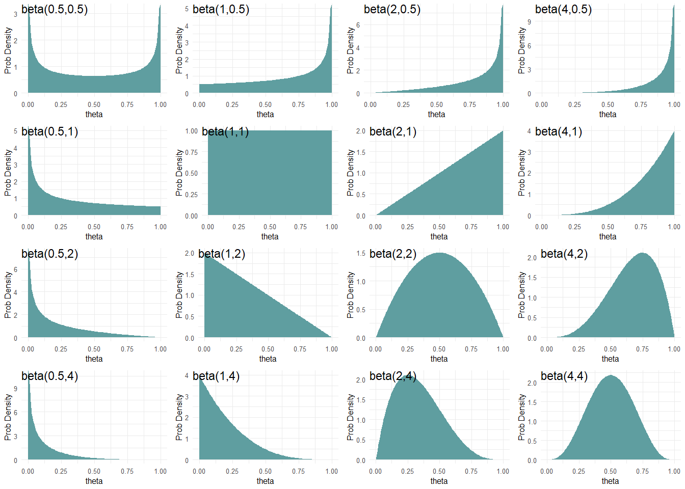
Figure 6.7 shows beta distributions for various \(\alpha\) and \(\beta\) parameter values. From Figure 6.7, we see the \(\textrm{beta}\) distribution is flexible in showing a variety of representations of our uncertainty. When looking at the distribution for \(\textrm{beta}(0.5,0.5)\) (top-left) we see that theta values closer to zero or one have higher density values than values closer to 0.5. At the other end, a \(\textrm{beta}(4,4)\) distribution places more plausibility for values closer to 0.5. In between, it seems distributions that favor high or low values for \(\theta\) can be constructed.
The \(\textrm{beta}\) distribution has a very neat property which can aid your selection of parameters to model your uncertainty:
you can roughly interpret \(\alpha\) and \(\beta\) as previously observed data where the \(\alpha\) parameter is the number of successes you have observed and the \(\beta\) parameter is the number of failures.
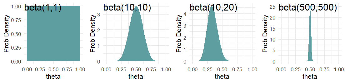
A beta(1,1) distribution is mathematically equivalent to a Uniform(0,1) distribution.
Hence, a \(\textrm{beta}(1,1)\) distribution can be thought of as saying a single success and failure have been witnessed, but we are completely unsure as to the probability of each. Whereas, a \(\textrm{beta}(10,10)\) distribution is like suggesting you have seen 20 outcomes and they have been split down the middle - i.e. you have observed some small evidence that the two outcomes occur in equal proportions. Another distribution, say \(\textrm{beta}(10,20)\), can indicate a belief that would accompany having seen 30 outcomes where failures occur 2 times as frequently as successes. Finally, a distribution like \(\textrm{beta}(500,500)\) might be used to represent your uncertainty in the flip of a fair coin. Figure 6.8 shows these four distributions (i.e. probability density functions) side-by-side.
Moving forward, we will often use the \(\textrm{beta}\) distribution to represent our prior beliefs regarding a probability. The support is \((0,1)\) and it is able to adopt some flexible shapes. Take a moment and confirm that you can answer these thought questions:
THOUGHT Question: Let theta represent the probability of heads on a coin flip. Which distribution, beta(0.5,0.5), beta(1,1), beta(2,2), beta(50,100) or beta(500,500) best represents your belief in theta given that the coin is randomly chosen from someone’s pocket?
THOUGHT Question: Which distribution, beta(0.5,0.5), beta(1,1), beta(2,2), beta(50,100), or beta(500,500) best represents your belief in theta given the coin is purchased from a magic store and you have strong reason to believe that both sides are heads or both sides are tails?
6.5 Questions to Learn From
See CANVAS.