7 Bayesian Inference On Graphical Models By Hand

Suppose some dark night a policeman walks down a street, apparently deserted; but suddenly he hears a burglar alarm, looks across the street, and sees a jewelry store with a broken window. Then a gentleman wearing a mask comes crawling out through the broken window, carrying a bag which turns out to be full of expensive jewelry. The policeman doesn’t hesitate at all in deciding that this gentleman is dishonest. But by what reasoning process does he arrive at this conclusion? … A moment’s thought makes it clear that our policeman’s conclusion was not a logical deduction from the evidence; for there may have been a perfectly innocent explanation for everything. It might be, for example, that this gentleman was the owner of the jewelry store and he was coming home from a masquerade party, and didn’t have the key with him. But just as he walked by his store a passing truck threw a stone through the window; and he was only protecting his own property. Now while the policeman’s reasoning process was not logical deduction, we will grant that it had a certain degree of validity. The evidence did not make the gentleman’s dishonesty certain, but it did make it extremely plausible. (- Jaynes 2003)
Jaynes, Edwin T. 2003. Probability Theory: The Logic of Science. Cambridge university press.
In the above story, the policeman used what we call plausible reasoning - an allocation of credibility to all possible explanations for his observations. While yes, just maybe, a masquerade party explains the man’s outfit - more likely, the model that best explains all of the collected data is that this is a robbery in progress.
In this book, our version of plausible reasoning is called Bayesian inference - a methodology for updating our mathematical representations of the world - or small pieces of the world - as more data becomes available.
7.1 An Illustrative Example

Figure 7.1 shows a sample of how Chili’s restaurants were refreshing their stores’ look and feel. You can imagine that through this investment Chili’s expects to increase store traffic. Let’s walk through a hypothetical argument between two managers as to the effect of this type of investment.
Assume the two managers have competing models for what effect a proposed Chili’s exterior remodel will have on its stores:
- The Optimist Model (Model1) : This model is from a manager who is very excited about the effect of exterior renovations and argues that 70% of all Chili’s stores will see at least a 5% increase in sales.
- The Pessimist Model (Model2) : This model is from a manager who felt the old facade was still fresh. This manager argues that only 20% of all Chili’s stores will see at least a 5% increase in sales.
These managers recognize and respect their differing opinions - they agree to test the remodel in a randomly chosen store. They hire you as a business data analyst and ask you to make the decision as to whose model is more right in light of the test’s results. Your job is to allocate credibility to the two competing models both before seeing results and after seeing results. Initially, you might not have any reason to favor one model over another, but as data is collected, your belief in whose model is more believable will change. For example, if the tested store sales decrease, then the pessimist model would seem more credible. Quantifying - using probability - how to allocate plausibility both with and without data is your task.
7.2 Building A Graphical Model of the Real-World
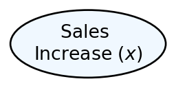
The first step is to create a graphical model representation of the Chili’s question. Starting simple, let’s only imagine that we test the remodel in one store and our single data point (i.e. whether the one tested store increases sales or not) follows a Bernoulli distribution. The graphical model is simply the random variable oval:
And, the statistical model is represented like this:
You might notice that theta or other greek letters because the computational world does not make the actual greek letters like
**We will explore the more realistic case of multiple and infinite possiblities for
Great, we have seen this model before when representing coin flips. Our data is analogous to heads or tails of a coin flip. The data will be reduced to a zero or one for each store. If given numpy.random.default_rng().binomial(n,p,size), but, we do not know
From the managerial story above,
See https://youtu.be/nCRTuwCdmP0 for gaining some intuition about prior probabilities.
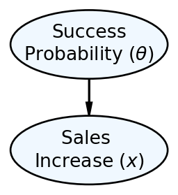
So now, we can more completely specify our data story using both a graphical and a statistical model with specified prior probabilities. The graphical model we would use to communicate with stakeholders is now two ovals representing our uncertainty in the probability of success and the observed sales increase (random variable math-labels for
And, the statistical model is represented like this:
where the prior probability distribution for
Two main classes of statistical models exist. A generative model can be used to generate random data as it gives a full probabilistic recipe (i.e. a joint distribution) for creating random data. In contrast, a discriminative model classifies or predicts without the ability to simulate all the random variables of the model.
Figure 7.3 and the accompanying statistical model represents a generative model. A crude definition of a generative model is that it is a recipe for simulating real-world data observations. In this case, simulating a single store’s success mimics a top-down reading of Figure 7.3:
- Simulate a potential success probability by randomly picking, with equal probability, either the optimist (
- Simulate a store’s success by using the probability from (1) and generating a Bernoulli random variable with that probability of success (
We can easily show how to simulate an observation by writing code for the recipe:
from numpy.random import default_rng
import numpy as np
rng = default_rng(seed=123456)

# Generate Which Manager Model is Correct
# map theta = 70% to the number 1 and
# map theta = 20% to the number 0.
sampleModel = rng.binomial(n=1, p=0.5, size = 1)
theta = np.where(sampleModel == 1, 0.7, 0.2)

print(theta)

# Generate 20 sample stores for that theta[0.7]rng.binomial(n=1, p=theta, size = 20)array([1, 1, 0, 0, 1, 1, 1, 0, 0, 1, 1, 1, 1, 1, 1, 0, 1, 1, 1, 1],
dtype=int64)The above simulated that
Key Concept: Much of your subsequent work in this course will use this notion of generative models as recipes. You will 1) create generative models that serve as skeleton recipes - recipes with named probability distributions and unknown parameters - for how real-world data arises, and 2) inform models with data by reallocating plausibility to the recipe parameters that are most consistent with the data. In the above, had the value of theta been hidden from you, you would be able to guess it from the data; most of the 20 stores succeeded in the simulation.
A guiding principle for creating good generative models is that the generated data should mimic data that you, as a business data analyst, believe is plausible. If the generative model outputs implausible data in high frequency, then your model is not capturing the essence of the underlying data story; your modelling assumptions will need work. When the generative model seems correct in the absence of data, then data can feed the updating process (to be explored in Section 7.4 which sensibly reallocates prior probability so that model parameters that tend to generate data similar to the observed data are deemed more plausible.
7.3 From Model To Joint Distribution
The graphical model of Figure 7.3 shows that we have uncertainty about two related random variables: 1) Success Probability (
Prior to data collection, we know (based on assumptions) a few things must be true:
If you are rusty on your defintion of conditional probability, take a moment to refresh yourself by viewing this set of videos from Khan Academy: Khan Academy’s calculating conditional probability.
- One of the four scenarios must be true, thus
- Equal probability is given to the possible models such that
- Assuming any model is true, then we know the conditional probability of success - i.e.
- If we apply the definition of conditional probability - i.e.
- The marginal probability of success (i.e. the probabilty of success without reference to the model) is the sum of the first row’s elements:
- The marginal probability of failure (i.e. the probabilty of failure without reference to the model) is the sum of the second row’s elements:
Taken together, the above truths enable us to fully specify the marginal distributions
When you see something like
In data analysis, we are always interested in updating our beliefs about
7.4 Bayesian Updating Of The Joint Distribution
Our generative model recipe led us to this prior joint distribution for
Inference is the process of reallocating prior probability in models based on observed data, i.e. determining
7.4.1 A Quick Derivation of Bayes Rule
From the definition of conditional probability, we know that
Thus, by simple mathematical manipulation of the last equality we get Bayes rule:
Since A and B are somewhat arbitrary, let’s relate Bayes Rule to the concept of collecting data to reallocate probability among competing models:
7.4.2 Using Bayes Rule
The mathematics of Bayes rule might seem intimidating, but showing how Bayes rule works using our joint distribution table can make it more intuitive. Let’s assume the first store is a success - sales increase by more than 5%. Thus, we no longer need to worry about the case of
Once zoomed in on this row, we need to re-allocate 100% of our plausability measure to just this row because we are 100% certain it happened. Intuitively, it seems that the updated plausibility allocated to each model should be proportional to our prior beliefs in each model - and this is actually what the mathematics of Bayes rule does. To make the success row sum to 1 instead of
See the Khan Academy video on dividing fractions if you need a refresher.
and
A good check that you did the Bayes rule math correctly is to ensure your posterior probabilities sum to 1 (i.e.
Bayes rule takes some working with it to fully digest. Spend a moment to make sure you know where each part of the above Bayesian updating calculation comes from. The components of a Bayes rule calculation are frequently referred to and each one has a special name:
- Prior -
- Likelihood -
- Evidence or Marginal Likelihood -
- Posterior -
Thus, Bayes rule restated for data analysis purposes:
and it shows exactly how we update our prior original assumptions
7.5 Inference Summary So Far
The steps for initially allocating and then, reallocating probability in light of data are to:
- Make A Graphical Model - Construct plausible relationships among the inter-related random variables of interest - in this chapter’s example the two random variables were
- Provide Prior Probabilities Via A Statistical Model - Create prior probabilities to ensure that your model can generate seemingly plausible data. Our prior was easy to figure out (50%/50%) based on the context, but in future chapters we will explore more complex scenarios.
- Update Using Bayes Rule - Use Bayesian updating to process data and reallocate probability among the competing models. So far, we learned to do this mathematically, but we will leverage the power of Python and its packages to make the computer do this tedious work for us.
When additional data is received, please know that Bayes rule still works. Just take the posterior output from the original data, and then use that as your prior when digesting the new information. Equivalently, you can just update the original prior with the combined set of original data and new data. Either way, Bayes rule will yield the same results.
While the math may seem tedious now, we are actually learning the math now to move away from it in the future; once we understand how the math works, we can leverage computation to do the math for us with a deeper understanding of what the computation does.
7.6 Questions to Learn From
See CANVAS.