9 Probability Distributions for Representing Priors and Data Generation

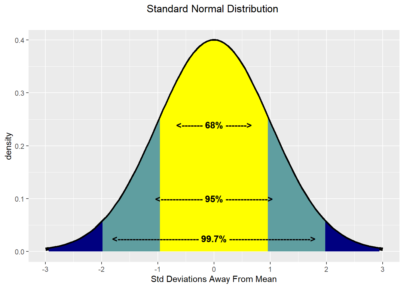
In this chapter, we move beyond $Bernoulli$ data and the small selection of prior distributions that you have been exposed to. We now look at multiple distributions that can serve as prior distributions, data distributions, or both.

9.1 Normal Distribution

The $normal$ distribution also known as the Gaussian is perhaps the most well-known distribution. The $normal$ distribution is typically notated as $N (μ, σ)$ and has two parameters:

More details for the $normal$ distribution available at https://en.wikipedia.org/wiki/Normal_distribution.

$μ$ : the mean or central tendency of either your data generating process or your prior uncertainty and,
$σ$ : a measure of spread/uncertainty around $μ$ . Note that for all normally distributed random variables that $\approx$ 95% of realizations fall within a $2 σ$ band around $μ$ (i.e. if $X \sim N (μ, σ)$ , then $P (μ - 2 σ \leq x \leq μ + 2 σ) \approx 95 %$ ) and $\approx$ 99.7% of realizations fall within a $3 σ$ band (See Figure 9.1).

Figure 9.1: Demonstrating the relationship between the standard deviation and the mean of the normal distribution.

There is an astounding amount of data in the world that appears to be normally distributed. Here are some examples:

Finance: Changes in the logarithm of exchange rates, price indices, and stock market indices are assumed normal
Testing: Standardized test scores (e.g. IQ, SAT Scores)
Biology: Heights of males in the united states
Physics: Density of an electron cloud is 1s state.
Manufacturing: Height of a scooter’s steering support
Inventory Control: Demand for chicken noodle soup from a distribution center

Due to its prevalance and some nice mathematical properties, this is often the distribution you learn the most about in a statistics course. For us, it is often a good distribution when data or uncertainty is characterized by diminishing probability as potential realizations get further away from the mean. Given the small probability given to outliers, this is not the best distribution to use (at least by itself) if data far from the mean are expected. Even though mathematical theory tells us the support of the $normal$ distribution is $(- \infty, \infty)$ , the probability of deviations far from the mean is practically zero. As such, do not use the $normal$ distribution by itself to model data with outliers.

Here is just a sample of three normal distributions:

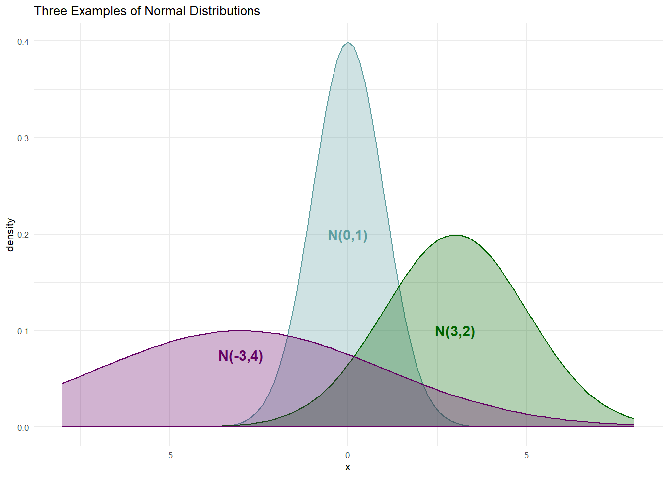
Figure 9.2: Example probability densities of the normal distribution.}

The densities of Figure 9.2 show the typical bell-shaped, symmetric curve, that we are used to. Since the $normal$ distribution has two parameters, the graphical model representing our uncertainty in the generating process for normally distributed data will have three random variables (see Figure 9.3): 1) the observed data, 2) the mean $μ$ , and 3) the standard deviation $σ$ .

Figure 9.3: Simple model with observed normal data whose likelihood is parametrized by mu and sigma. Priors for mu and sigma, the parameters, will need to be defined to have a complete generative model.

and the statistical model with priors:

$\begin{aligned} X \sim & N (μ, σ) \\ μ \sim & Some Prior Distribution \\ σ \sim & Some Prior Distribution \end{aligned}$

where the prior distributions get determined based on the context of the problem under study.

For example, let’s say we are interested in modelling the heights of cherry trees. Even if we do not know much about cherry trees, we can probably be 95% confident that they are somewhere between 1 foot and 99 feet. Hence, we can set up a prior with 95% probability between 1 and 99, i.e. if $X \equiv Cherry Tree Height$ , then we know that $P (μ - 2 σ \leq x \leq μ + 2 σ) \approx 95 %$ . Hence, we can select $μ \sim N (50, 24.5)$ . Note this is a prior on the average height, not the individual height of a cherry tree.

Choosing a prior on $σ$ is less intuitive. What do we know about the variation in heights of individual trees? Not much. We can probably bound it though. In fact, we can be 100% certain this is greater than zero; no two cherry trees will be the same height. And I am confident, that cherry tree heights will most definitely fall within say 50 feet of the average, so let’s go with a uniform distribution bounded by 0 and 50.

Hence, our statistical model becomes:

$\begin{aligned} X \sim & N (μ, σ) \\ μ \sim & N (50, 24.5) \\ σ \sim & Uniform (0, 50) \end{aligned}$

After choosing our prior, we then use data to reallocate plausibility over all our model parameters. There is a dataset available with this book of cherry tree heights:

## get cherry tree data
import pandas as pd
import xarray as xr
import numpy as np

# Source: Ryan, T. A., Joiner, B. L. and Ryan, B. F. (1976) 
# The Minitab Student Handbook. Duxbury Press.

## This data set provides measurements of the diameter (girth), height,
## and volume of timber in 31 felled black cherry trees. 
url = "https://raw.githubusercontent.com/flyaflya/persuasive/main/trees.csv"
treesDF = pd.read_csv(url)
## make tree height an array
## numpyro will NOT accept a pandas series as input
treeHeightData = treesDF.Height.to_numpy() # series to numpy array

which we can use to create code to get a posterior. Using numpyro, we get our representative sample of the posterior distribution:

import numpyro
import numpyro.distributions as dist
from jax import random
from numpyro.infer import MCMC, NUTS
import arviz as az

## make tree height an array - numpyro will NOT accept a pandas series as input
treeHeightData = treesDF.Height.to_numpy() # series to numpy array

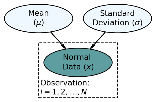
## define the graphical/statistical model as a Python function
def cherryTreeModel(x):
    # loc – mean of the distribution (often referred to as mu)
    # scale – standard dev. of the distribution (often referred to as sigma)
    mu = numpyro.sample('mu', dist.Normal(loc = 50, scale = 24.5))
    sigma = numpyro.sample('sigma', dist.Uniform(low = 0, high = 50))
    with numpyro.plate('observation', len(x)):
        x = numpyro.sample('x', dist.Normal(loc = mu, scale = sigma), obs=x)

# ## computationally get posterior distribution
mcmc = MCMC(NUTS(cherryTreeModel), num_warmup=1000, num_samples=4000) 
rng_key = random.PRNGKey(seed = 111) ## so you and I get same results
mcmc.run(rng_key, x=treeHeightData) ## get representative sample of posterior

drawsDS = az.from_numpyro(mcmc).posterior ## get samples into xarray

And then, plot the credible values using the plot_posterior() function from the arviz package. The posterior distribution provides representative samples of all unobserved parameters in the model. For each parameter, the 94% highest density interval (HDI) is presented (94% is a changeable default). This interval represents the smallest interval such that 94% of all sample draws fall within the range of values spanned by the horizontal black line. The numbers above the black line are rounded approximations for the interval boundaries. The hdi function could yield exact results:

az.hdi(drawsDS,hdi_prob = 0.94)

where we see plausible values for expected cherry tree height $μ$ are between 73.6 and 78.2.

REMINDER: the posterior distribution for the average cherry tree height is no longer normally distributed and the standard deviation is no longer uniform. This is a reminder that prior distribution families do not restrict the shape of the posterior distribution.

We now have insight as to the height of cherry trees as our prior uncertainty is significantly reduced. Instead of cherry tree heights averaging anywhere from 1 to 99 feet as accommodated by our prior, we now say (roughly speaking) the average height is somewhere in the 74-78 foot range. Instead of the variation in height of trees being plausibly as high as 50 feet, the height of any individual tree is most likely within 10-17 feet of the average height (i.e. $\approx μ \pm 2 σ$ ).

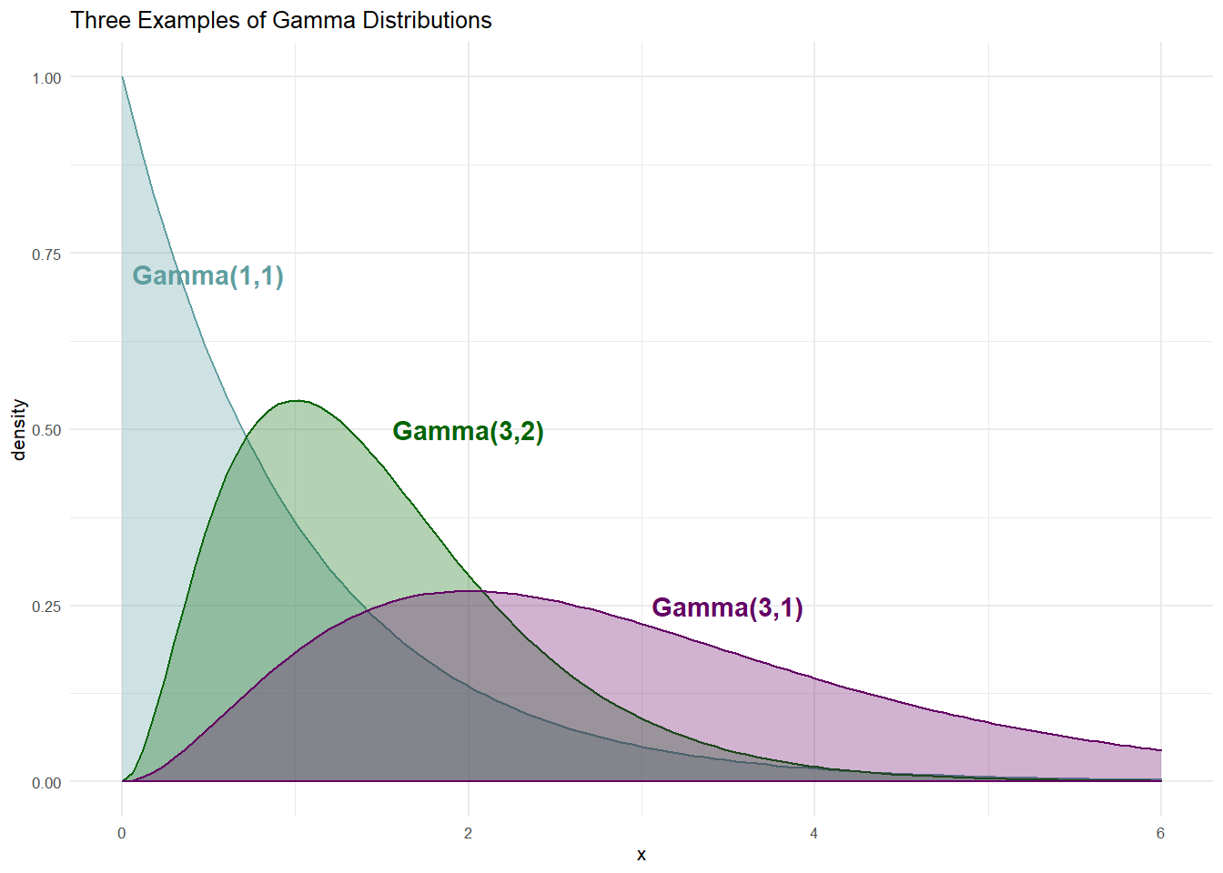
9.2 Gamma Distribution

The support of any random variable with a normal distribution is $(- \infty, \infty)$ which means just about any value is theoretically possible - although values far away from the mean are practically impossible. Sometimes, you want a similar distribution, but one that has constrained support of $(0, \infty)$ , i.e. the data is restricted to being strictly positive (even 0 has no density). The $gamma$ distribution has such support. While the $gamma$ distribution is often used to fit real-world data like total insurance claims and total rainfall, we will often use this distribution as a prior for another distribution’s parameters. For example, the standard deviation of a normally distributed random variable is strictly positive, so the gamma is often appropriate for modelling uncertainty in a standard deviation parameter. Let’s take a deeper look.

More details for the $gamma$ distribution available at https://en.wikipedia.org/wiki/Gamma_distribution.

The $gamma$ distribution is a two-parameter distribution notated $gamma (α, β)$ . While there are other ways to specify the two parameters, we will use the convention that $α$ refers to a shape parameter (numpyro uses the term concentration parameter) and $β$ a rate parameter. An intuitive meaning of shape and rate is beyond our needs at this point, for now we just learn those terms because numpyro expects these two parameters when using a $gamma$ distribution. Here are some examples of $gamma$ distributions to get a feel for its shape:

Figure 9.4: Example probability densities of the gamma distribution.

When choosing $α$ and $β$ so that our prior uncertainty is accurately represented, we will use a few mathematical properties of the gamma distribution. Assuming $X \sim gamma (α, β)$ , the following properties are true:

$E [X] = \frac{α}{β}$ : The mean of a gamma-distributed random variable is the ratio of $α$ over $β$
$Var [X] = \frac{α}{β^{2}}$ : The variance, a popular measure of spread or dispersion, can also be expressed as a ratio of the two parameters.

The Gamma distribution is a superset of some other famous distributions. The $Exponential$ distribution can be expressed as $Gamma (1, λ)$ and the $Chi-Squared$ distribution with $ν$ degrees of freedom can be expressed as $Gamma (\frac{ν}{2}, \frac{1}{2})$ .

These properties will be demonstrated when the gamma is called upon as a prior in subsequent sections.

9.3 Student t Distribution

For our purposes, the $Student t$ distribution is a normal distribution with fatter tails - i.e. it places more plausibility to values far from the mean than a similar $normal$ distribution would. Whereas estimates for the mean of a $normal$ distribution get pulled towards outliers, the $Student t$ distribution is less susceptible to that issue. Hence, for just about all practical questions, the $Student t$ is a more robust distribution both as likelihood and for expressing prior uncertainty. I would almost always prefer it to a normal distribution with the exception that one extra parameter needs to be managed.

The $Student t$ distribution, as parameterized in numpyro, is a three parameter distribution; notated $Student-t (ν, μ, σ)$ . The last two parameters, $μ$ (i.e. loc) and $σ$ (i.e. scale), can be interpreted just as they are with the normal distribution. The first parameter, $ν$ (greek letter pronounced “new”, phonetically spelled “nu”, and represented in numpyro as df), refers to the degrees of freedom. Interestingly, as $ν \to \infty$ (i.e. as $ν$ gets large) the $Student t$ distribution and the normal distribution become identical; in other words, the fatter tails go away. For all of our purposes, we use a gamma prior for representing our uncertainty in $ν$ as recommended in https://github.com/stan-dev/stan/wiki/Prior-Choice-Recommendations.

Here is a sample of three student-t distributions:

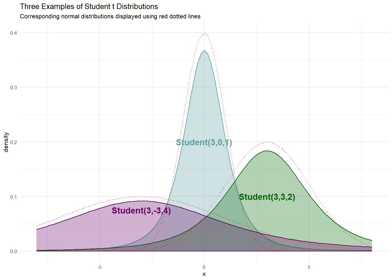
Figure 9.5: Example probability densities of the Student t distribution.

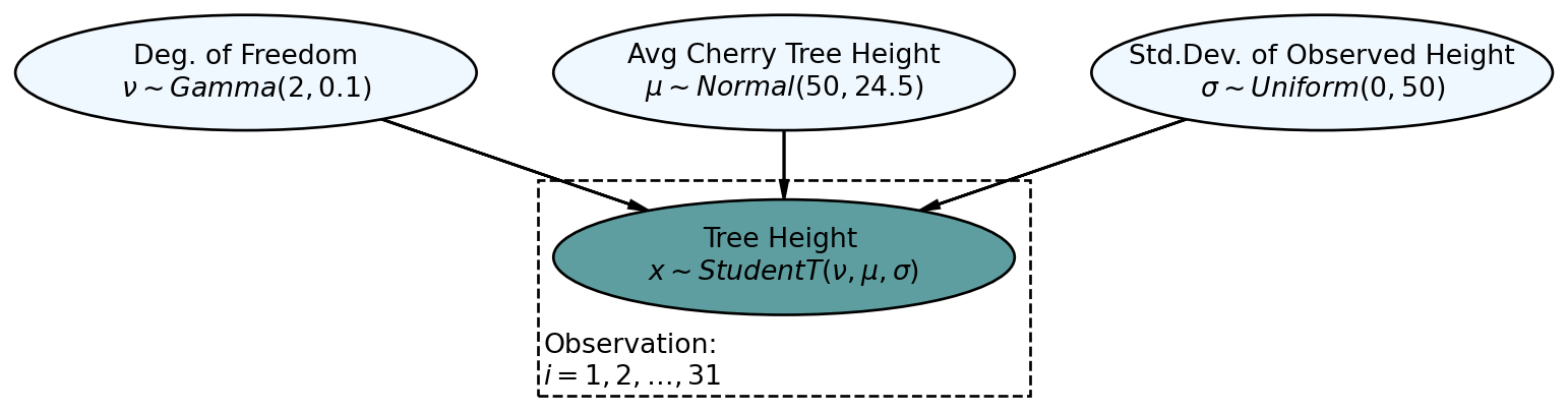
If we wanted to model the cherry tree heights using a $Student t$ distribution instead of a $normal$ distribution, the following generative DAG (i.e. combined graphical + statistical model) can be used:

Figure 9.6: Simple model with observed student-t data whose likelihood is parametrized by nu, mu, and sigma. Specified yriors for all parameters make this a complete generative model.

Using numpyro, we get our representative sample of the posterior:

## define the generative DAG as a Python function
def cherryTreeModelT(x):
    # df - degrees of freedom (often referred to as nu)
    # loc – mean of the distribution (often referred to as mu)
    # scale – standard dev. of the distribution (often referred to as sigma)
    nu = numpyro.sample('nu', dist.Gamma(concentration = 2, rate = 0.1))
    mu = numpyro.sample('mu', dist.Normal(loc = 50, scale = 24.5))
    sigma = numpyro.sample('sigma', dist.Uniform(low = 0, high = 50))
    with numpyro.plate('observation', len(x)):
        x = numpyro.sample('x', dist.StudentT(df = nu, 
                                              loc = mu, 
                                              scale = sigma), 
                           obs=x)

# ## computationally get posterior distribution
mcmc = MCMC(NUTS(cherryTreeModelT), num_warmup=1000, num_samples=4000) 
rng_key = random.PRNGKey(seed = 111) ## so you and I get same results
mcmc.run(rng_key, x=treeHeightData) ## get representative sample of posterior

drawsDS = az.from_numpyro(mcmc).posterior ## get posterior samples into xarray

And then, plot the credible values to observe very similar results, at least for $μ$ and $σ$ , as the results seen using the $normal$ distribution:

az.plot_posterior(drawsDS)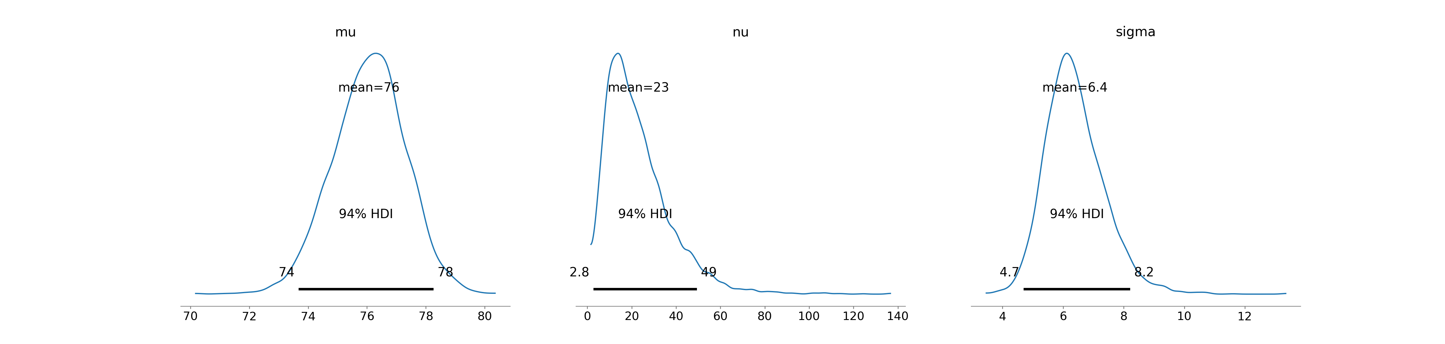

Figure 9.7: Posterior distribution for the mean, standard deviation, and degrees of freedom when modelling cherry tree heights.

The wide distribution for $ν$ can be interpreted as saying we do not know how fat the tails for this distribution should be. Which actually makes sense! You need a lot of data to potentially observe outliers, so with only 31 observations our generative model remains uncertain about this degrees of freedom parameter.

9.3.1 Robustness Of Student t Distribution

To highlight the robustness of the $Student-t$ distribution to outliers and the lack of robustness of the $normal$ distribution, let’s add a mis-measured cherry tree height to the data. While most heights are between 60-80 feet, a mis-measured and truly unbelievable cherry tree height of 1,000 feet is added to the data (i.e. treeHeightDataWithOutlier = np.append(treeHeightData,1000)). Figure 9.8 shows recalculated posterior densities for both the normal and student t priors.

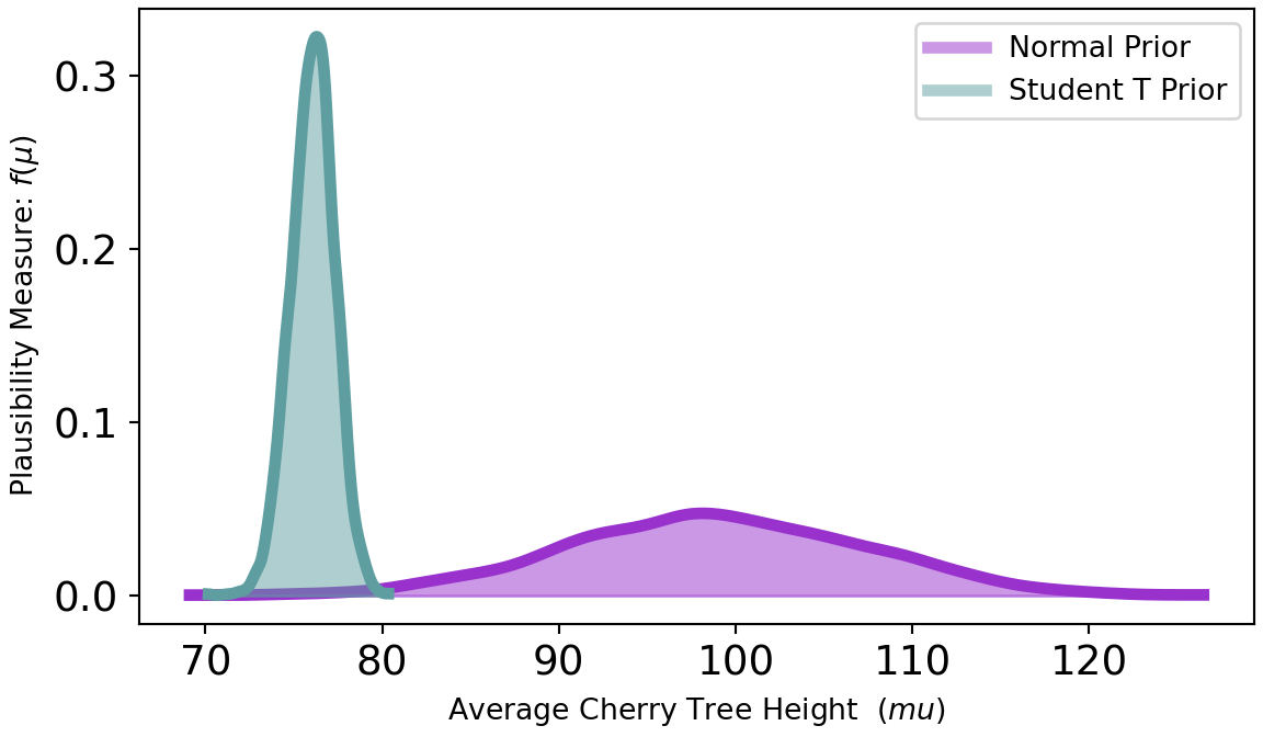
Figure 9.8: Estimates of a distributions central tendency can be made to downplay outliers by using a student t prior distribution for the mean. Normal distribution as a prior is more affected by outlier datapoints and the mean no longer represents a typical cherry tree height.

As seen in Figure 9.8, the posterior estimate of the mean $μ$ when using a $normal$ prior is greatly affected by the outlier data point - the posterior average height gets concentrated around an absurd 100 feet. Whereas, the $Student-t$ prior seems to correctly ignore that mis-measured data and concentrates the posterior expectation of average cherry tree height around 76 (as discovered previously). While in this case, ignoring the outliers is desirable and the Student-T distribution provides a robust method for discounting outliers, all modelling choices should be made so that the posterior distribution accurately reflects your prior expectations of how data should be mixed with prior knowledge.

9.4 Poisson Distribution

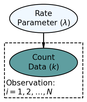
The Poisson distribution is useful for modelling the number of times an event occurs within a specified time interval. It is a one parameter distribution where if $K \sim Poisson (λ)$ , then any realization $k$ represents the number of times an event occurred in an interval. The parameter, $λ$ , has a nice property in that it is a rate parameter representing the average number of times an event occurs in a given interval. Given this interpretability, estimating this parameter is often of interest. A graphical model for estimating a Poisson rate parameter from count data is shown in Figure 9.9.

Figure 9.9: A typical generative model for count datauses a Poisson data distribution with rate parameter lambda.

and a prior for $λ$ will be determined by the use case. $^{* *}$ For example, we can retrieve a dataset of 55,167 (daily) observations of the number of tickets written by NYC police precincts. This data is modified from (a conference talk)[https://github.com/stan-dev/stancon_talks/tree/master/2018/Contributed-Talks/01_auerbach] which originally sourced data from https://opendata.cityofnewyork.us/.

There are several assumptions about Poisson random variables that dictate the appropriateness of modelling counts using a Poisson random variable. Three of those assumptions are: 1) $k$ is a non-negative integer of counts in a specified time interval, 2) the rate at which events occur is constant, and 3) the occurrence of one event does not affect the probability of additional events occurring (i.e. events are independent). As an example of violating the second assumption, it would not be appropriate to model arrivals per hour to a restaurant as a Poisson random variable because the rate of arrivals certainly varies with time of day (e.g. lunch, dinner, etc.)

url = "https://raw.githubusercontent.com/flyaflya/persuasive/main/tickets.csv"
ticketsDF = pd.read_csv(url, parse_dates = ["date"])
ticketsDF.head(5)

   precinct       date month_year  daily_tickets
0         1 2014-01-01    01-2014             17
1         1 2014-01-02    01-2014             67
2         1 2014-01-03    01-2014             17
3         1 2014-01-04    01-2014             42
4         1 2014-01-05    01-2014             54

Let’s use the above data to look at tickets issued only on Wednesdays in New York City, and then we will model the rate of ticketing on Wednesdays using the Poisson likelihood with appropriate prior. Our restriction to Wednesday is based on our knowledge that there may be daily fluctuations in ticketing rates; for example, maybe weekends are slower ticketing days. By restricting our analysis to one day of the week, we have a better chance at conforming to the assumption of a Poisson random variable that the expected rate at which events occurs is constant throughout the time period of analysis; note, the arrivals need not occur at constant intervals, just the average rate of arrival should not change.

## get count data of tickets for Wednesdays only
## aggregate data across precincts
wedTicketsDF = (
    ticketsDF
    .assign(dayOfWeek = lambda DF: DF.date.dt.day_name())
    .where(lambda DF: DF.dayOfWeek == "Wednesday")
    .dropna()
    .groupby("date")
    .agg(numTickets = ('daily_tickets', 'sum'))
)

A quick visualization of the data, Figure 9.10, shows some outliers. This is usually not a good sign to use a Poisson distribution, but we will continue blissfully unaware of the dangers (these dangers do get corrected in the next chapter).

plt.style.use("seaborn-whitegrid")
fig, ax = plt.subplots(figsize=(6, 3.5), 
                        layout='constrained')
ax.scatter(wedTicketsDF.index, wedTicketsDF.numTickets)
ax.set_xlabel("Date")
ax.set_ylabel("# of Tickets Issued")
ax.set_title("Tickets Issued on Wednesdays In New York City")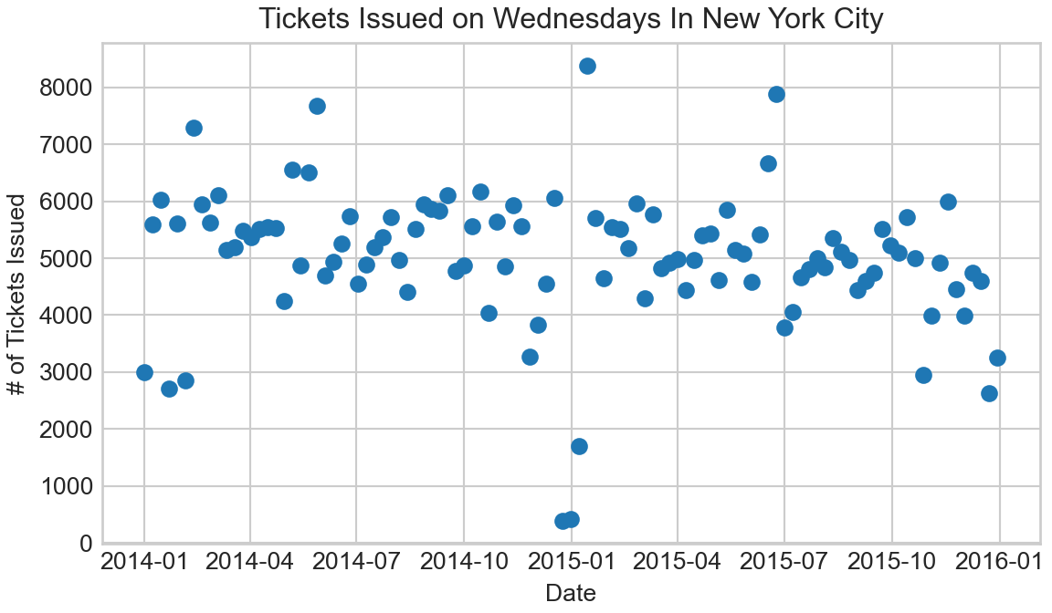

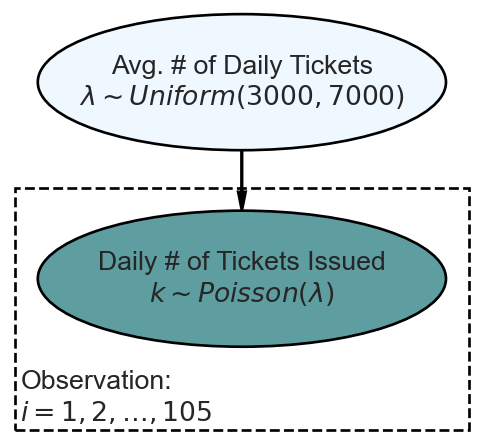
Figure 9.10: The number of daily traffic tickets issued in New York city from 2014-15.

Now, we model these two years of observations using a Poisson likelihood and a prior that reflects beliefs that the average number of tickets issued on any Wednesday in NYC is somewhere between 3,000 and 7,000; for simplicity, let’s choose a $Uniform (3000, 7000)$ prior as in the generative DAG of Figure 9.11.

Figure 9.11: A generative DAG for modelling the daily issuing of tickets on Wednesdays in New York city.

And extracting our posterior for the average rate of ticket issuance, $λ$ , yields the following posterior:

import xarray as xr
## make tickets data into an array - use xarray this time to show option
wedTicketsDS = xr.Dataset.from_dataframe(wedTicketsDF)
wedTickets = wedTicketsDS.numTickets.to_numpy()

## define the graphical/statistical model as a Python function
def ticketsModel(k):
    ## NOTE LAMBDA IS RESERVED WORD IN PYTHON... MUST USE MODIFIED NAME
    lambdaParam = numpyro.sample('lambdaParam', dist.Uniform(low = 3000, high = 7000))
    
    with numpyro.plate('observation', len(k)):
        k = numpyro.sample('k', dist.Poisson(rate = lambdaParam), obs = k)

# ## computationally get posterior distribution
mcmc = MCMC(NUTS(ticketsModel), num_warmup=1000, num_samples=4000) 
rng_key = random.PRNGKey(seed = 111) ## so you and I get same results
mcmc.run(rng_key, k=wedTickets) ## get representative sample of posterior

drawsDS = az.from_numpyro(mcmc).posterior ## get posterior samples into xarray
az.plot_posterior(drawsDS)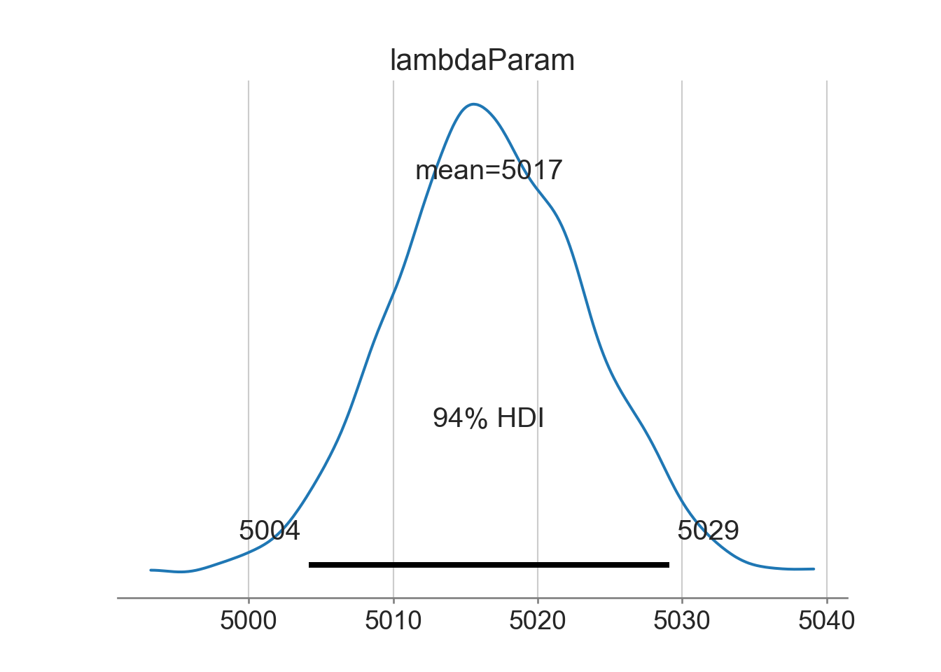

Figure 9.12: Posterior density for uncertainty in rate parameter lambda.

where we see that that the average rate of ticketing in NYC is slightly more than 5,000 tickets on each Wednesday. And just like always, you can use the posterior distribution to answer probabilistic queries. For example, we might want to know the probability that the average rate of ticketing is less than 5,000 (i.e. $P (λ < 5000)$ ):

(
    drawsDS
    .assign(lessThan5000Flag = lambda DS: DS.lambdaParam < 5000)
    .mean()
)

<xarray.Dataset>
Dimensions:           ()
Data variables:
    lambdaParam       float32 5.017e+03
    lessThan5000Flag  float64 0.00625

where the answer is $P (λ < 5000) \approx 1 %$ . Thus, we can confidently say that NYC pursues a strategy of at least 5,000 tickets per day on Wednesdays.

9.5 Getting Help

As important as it is, there is no perfect place to get information on mapping real-world phenomenon to probability distributions. Searching Wikipedia and YouTube are your best bets. After a few more chapters in this book, more complex model mappings will be accessible to you. Some of these complex modelling scenarios are available at the Stan website under case studies; the most accessible of them is this one about modelling golf putts, but it contains methods we have yet to learn. Another resource for future consumption (as it is more complex) is the Statistical Rethinking textbook with accompanying videos and translation into NumPyro code which is available here.

9.6 Questions to Learn From

See CANVAS.