8 Computational Bayesian Inference: Probabilistic Programming with NumPyro

In the Bayesian Inference chapter, we calculated (by hand) a posterior distribution using a single data point on whether the one tested Chili’s store increased sales. In this original Chili’s story, we limited ourselves to just two possible models of success:

The Pessimist Model: \(\theta = 20\)%
The Optimist Model: \(\theta = 70\)%

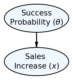
We represented the Chili’s narrative using the generative DAG shown in Figure 8.1 and got a posterior distribution, by hand, with just two candidate models, the pessimist model and the optimist model.

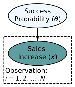
Figure 8.1: A model of how sales increases at Chili’s store are determined. First, a success probability is specified and then, the successfulness of a sales increase is determined as a function of the success probability.

We now expand our analysis to consider infinite possible values of success probability \(\theta\) where \(0 \leq \theta \leq 1\). This expansion can be expressed in an updated graphical model plus an updated statistical model. The updated graphical model is in Figure 8.2.

Figure 8.2: Adding darker fill to observed nodes and a plate to represent that N observations are being used to create a posterior for theta.

The updated statistical model is below.

In the above, \(\theta \sim \textrm{ Uniform}(0,1)\) becomes the new representation of our prior probability. This prior spreads equal plausibility among all potential values for probability \(\theta\). We are asserting that all probability values are equally likely. In the previous chapter, for any given \(\theta\) value, we were able to calculate prior and likelihood by hand, but now there are infinite \(\theta\) values.

To manually use Bayes rule to calculate the posterior distribution for the infinite possible values of \(\theta\) is impossible. That would simply take too long. Instead, we will rely on state-of-the-art computational techniques and software to deliver us a representative sample from the posterior distribution. In fact, the software we will use allows us tremendous flexibility; seemingly accommodating any probabilistic graphical model consisting of the most commonly used probability distributions. In other words, we as analysts supply a our model, prior, and some data, and then, the computer spits out the posterior - using Bayes rule behind the scenes to properly update our prior assumptions to place more plausibility on model parameters that are consistent with the observed data.

8.0.1 Bayesian Updating With NumPyro

Figure 8.3: The NumPyro logo. NumPyro calculates joint posterior distributions using an interface developed at Uber Labs and a numerical engine developed by Google.

NumPyro is an offshoot of Pyro, a universal probabilistic programming language (PPL) written in Python. We use NumPyro which uses Jax to gain a 100x speedup over Pyro (which used PyTorch) for the types of problems we will work on. You can read more about the origins of Pyro at https://www.uber.com/blog/pyro/.

To get the computer to do our work, we need to translate our data and generative DAG (i.e. graphical model + statistical model that has enough detail to simulate data) into a computational model (i.e. a computer-world model that calculates posterior distributions). We will learn to do this is using the fantastic numpyro package.

The following probability distributions (and more) are classes in the distributions sub-module of numpyro: Uniform, Normal, LogNormal, Bernoulli, Binomial, BetaBinomial, NegativeBinomial, Poisson, Gamma, InverseGamma, Weibull,Exponential, Pareto, StudentT, Laplace, Beta, Cauchy, Chi2, Logistic, MultivariateNormal, MultivariateStudentT,Multinomial, Categorical, Dirichlet, DirichletMultinomial, LKJ. Many of these will be introduced in subsequent chapters and all others can be found on Wikipedia. Do not let the fancy names scare you, they are just ways of compactly representing uncertainty.

Step 1 - Create a Python function that tells numpyro how to simulate all the nodes of your graphical model.

When reproducing a graphical and statistical model in numpyro code, the entire model gets defined as a function where the sole argument to the function (for now) is the observed data. Shown below is the coded representation of Figure 8.2:

import numpy as np
import numpyro
import numpyro.distributions as dist

## define the graphical/statistical model as a Python function
## pass data and the cardinality of plates as inputs
## N represents the number of chilis stores for which data is observed
def chilisModel(x):
    # numpyro.sample is a "primitive", i.e. basic building block of model
    theta = numpyro.sample('theta', dist.Uniform(low = 0, high = 1))
    # numpyro.plate is another primitive
    with numpyro.plate('N', len(x)):
        x = numpyro.sample('x', dist.Bernoulli(probs = theta), obs=x)

Two functions, called primitives, serve as building blocks in building the above function definition. They are:

numpyro.sample: This function takes two positional arguments and optionally one keyword argument. The first argument is simply the name of the node, I will use the mathematical shorthand name shown in the graphical model (e.g. theta or x). The second argument is the probability distribution that serves as either prior (for unobserved nodes) or likelihood (for observed nodes). The keyword argument obs is used to supply observed data when applicable, e.g. the sales outcomes of Chilis’ stores.
numpyro.plate: This function, typically used in the context of a with block takes two positional arguments. The first argument is simply the name of the plate, I will use the name of the plate shown in the graphical model (e.g. observation). The second argument is the cardinality of the plate which serves as a counter of how many individual realizations of each node are signified by their existence on the plate. In the above, the Sales Increase node is repeated once for every store that we observe data at.

When replicating a graphical and statistical model in code, all nodes that exist on a plate should be sampled within the context of that plate as signaled by indentation (just like is done in for loops). Additionally, all observed data should be passed into the function as arguments; above we pass in x as the lone argument.

Step 2 - Prepare Your Data.

Data should be passed in as either a numpy array or a jax.numpy array. In the above, we make up some data (1,1,0) to represent the first two stores successfully increasing sales and the third observed store failing to increase sales.

## define the required inputs for chilismodel
## assume first two stores are a success and 
## the third store is not (i.e. make up some data)
salesIncData = np.array([1,1,0])

Step 3 - Use NumPyro to Get A Representative Sample of The Posterior Distribution.

For now, I request that when you modify the below code for other problems, only modify the model name, i.e. chilisModel, and the arguments passed to mcmc.run. We will learn more details about this code in subsequent chapters. For now, let’s just digest the code at a high level of understanding where its purpose is to get a representative sample of unobserved parameters from the posterior distribution.

from jax import random
from numpyro.infer import MCMC, NUTS

## computationally get posterior distribution
## in the below line, only change "chilisModel" for different problems
mcmc = MCMC(NUTS(chilisModel), num_warmup=500, num_samples=4000) 
rng_key = random.PRNGKey(seed = 111) ## so you and I get same results
## supply the run method with a random key followed by arguments to model
mcmc.run(rng_key, x=salesIncData) ## get representative sample of posterior

The essence of the above code is that it creates an object called mcmc. A fancy algorithm called NUTS (No U-Turn Sampler) is set-up to create a representative sample of the posterior when passed some data. Data gets massed through the objects .run() method. The first argument to .run() is always a random key, and any additional arguments should pass data to the arguments of the NumPyro model.

After running mcmc.run(rng_key, x=salesIncData), the mcmc object has successfully created a representative sample from the posterior. This sample is often referred to as the posterior distribution. To access the posterior distribution, we will use functionality from the arviz package to extract an xarray dataset containing the information we need as shown below:

import arviz as az

## get samples into xarray
drawsDS = az.from_numpyro(mcmc).posterior
drawsDS

Step 4 - Use the posterior distribution for insight and for making probabilistic statements.

A quick and easy way to visualize the posterior distribution for theta is to use the arviz.plot_dist() function:

az.plot_dist(drawsDS.theta)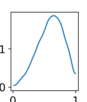

However, if you want to do any customization of an arviz plot, we must revert back to our typical matplotlib workflow and use arviz to modify an Axes object:

Figure 8.4: A probability density estimate of the posterior distribtuino for theta.

As can be seen from Figure 8.4, there is more plausibility to the right of 0.5. Hence, one might wonder “what is the probability that more than half the stores receiving a remodel will see a successful increase in sales?” To answer this, just like any probabilistic query, we use an indicator function and the fundamental bridge to find out:

## use indicator function to make probabilistic statements
## for example, find P(theta > 0.5)
(
    drawsDS
    .assign(thetaOver50 = drawsDS.theta > 0.50)
    .mean() # about 60% probability theta is over 50%
).to_pandas()

theta          0.599126
thetaOver50    0.699000
dtype: float64

Hence, we can say \(P(\theta>50\%) \approx 69\%\). You might also notice another result, namely \(\mathbb{E}[\Theta] \approx 60\%\). We will dive deeper into extracting insights in subsequent chapters. For now, the big takeaway is that data can be used to update our knowledge. Initially, we had complete uncertainty as to plausible values of \(\Theta\), but after observing just three stores, we refine our beliefs to shift plausibility away from extremely low-values which are inconsistent with the observed successes in store sales.

8.1 Using a beta Prior in NumPyro

Let’s now use a \(\textrm{beta}\) distribution prior to reenforce how NumPyro works, but more importantly to demonstrate how priors and data observations come together to make a posterior distribution.

Figure 8.5: Adding darker fill to observed nodes and a plate to represent that N observations are being used to create a posterior for theta.

The updated statistical model is below.

\[ \begin{aligned} \Theta \equiv& \textrm{ Store Success Probability: } \\ X \equiv& \textrm{ Sales Increase: } \\ & \textrm{ If sales increase more than 5} \% \textrm{, then }X=1 \textrm{ otherwise, }X=0.\\ \theta \sim & \textrm{ Beta}(2,2) \\ x \sim & \textrm{ Bernoulli}(\theta) \end{aligned} \] Figure 8.5 is a DAG declaring a \(\textrm{beta}(2,2)\) prior as representative of our uncertainty in \(\theta\). We aren’t saying too much with this prior. This is a weak prior because. as we will see, it will be easily overwhelmed by data; its just saying that two successes and two failures have been seen. Let’s then imagine processing new data where we observe 20 successes and only two failures. This data is highly consistent with a very large value for theta. We can intelligently combine prior and data using numpyro to get our posterior:

import numpy as np
import numpyro
import numpyro.distributions as dist
import arviz as az
from jax import random
from numpyro.infer import MCMC, NUTS

## define the data - 20 successes and 2 failures
successData = np.concatenate((np.repeat(1, 20), np.repeat(0,2)))

## define the graphical/statistical model as a Python function
def betaBernoulliModel(x):
    # concentration1: 1st concentration parameter (alpha) for the Beta dist.
    # think the higher alpha, the more concentrated theta values towards 1
    # concentration0: 2nd concentration parameter (beta) for the Beta dist.
    # think the higher beta, the more concentrated theta values towards 0
    theta = numpyro.sample('theta', dist.Beta(concentration1=2, #alpha
                                              concentration0=2)) #beta
    with numpyro.plate('observation', len(x)):
        x = numpyro.sample('x', dist.Bernoulli(probs = theta), obs=x)

## computationally get posterior distribution
mcmc = MCMC(NUTS(betaBernoulliModel), num_warmup=500, num_samples=4000) 
rng_key = random.PRNGKey(seed = 111) ## so you and I get same results
mcmc.run(rng_key, x=successData) ## get representative sample of posterior

drawsDS = az.from_numpyro(mcmc).posterior ## get samples into xarray

And once the posterior sample (drawsDS) is created, we can query the results and compare them to the \(\textrm{beta}(2,2)\) prior:

from matplotlib.lines import Line2D

fig, ax = plt.subplots(figsize=(6, 3.5), 
                        layout='constrained')

# plot density estimate, i.e. estimate of f(x)
az.plot_dist(drawsDS.theta, ax = ax, color = "darkorchid",
             plot_kwargs = {"zorder": 1, "linewidth": 4, "alpha": 0.5},
             fill_kwargs={"alpha": 0.5},
             quantiles=[.10, .50, .90])

# plot prior from rep sample
beta2_2_repSample = default_rng(seed=111).beta(2,2,50000)
az.plot_dist(beta2_2_repSample, ax = ax, color = "cadetblue",
             plot_kwargs = {"zorder": 1, "linewidth": 4, "alpha": 0.5},
             fill_kwargs={"alpha": 0.5},
             quantiles=[.10, .50, .90])

ax.set_xticks([0,.25,.5,.75,1])
ax.set_ylabel('Plausibility Measure: ' + r'$f_\Theta(\theta)$')
ax.set_xlabel(r'$\theta$')

custom_lines = [Line2D([0], [0], color = "darkorchid", lw=4, alpha = 0.5),
                Line2D([0], [0], color = "cadetblue", lw=4, alpha = 0.5)]
ax.legend(custom_lines, ['Posterior', 'Beta(2,2) Prior'], loc='upper left')

plt.show()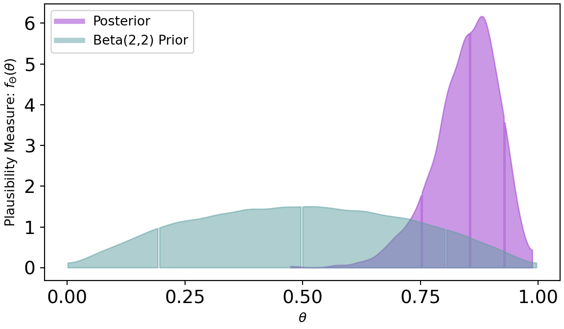

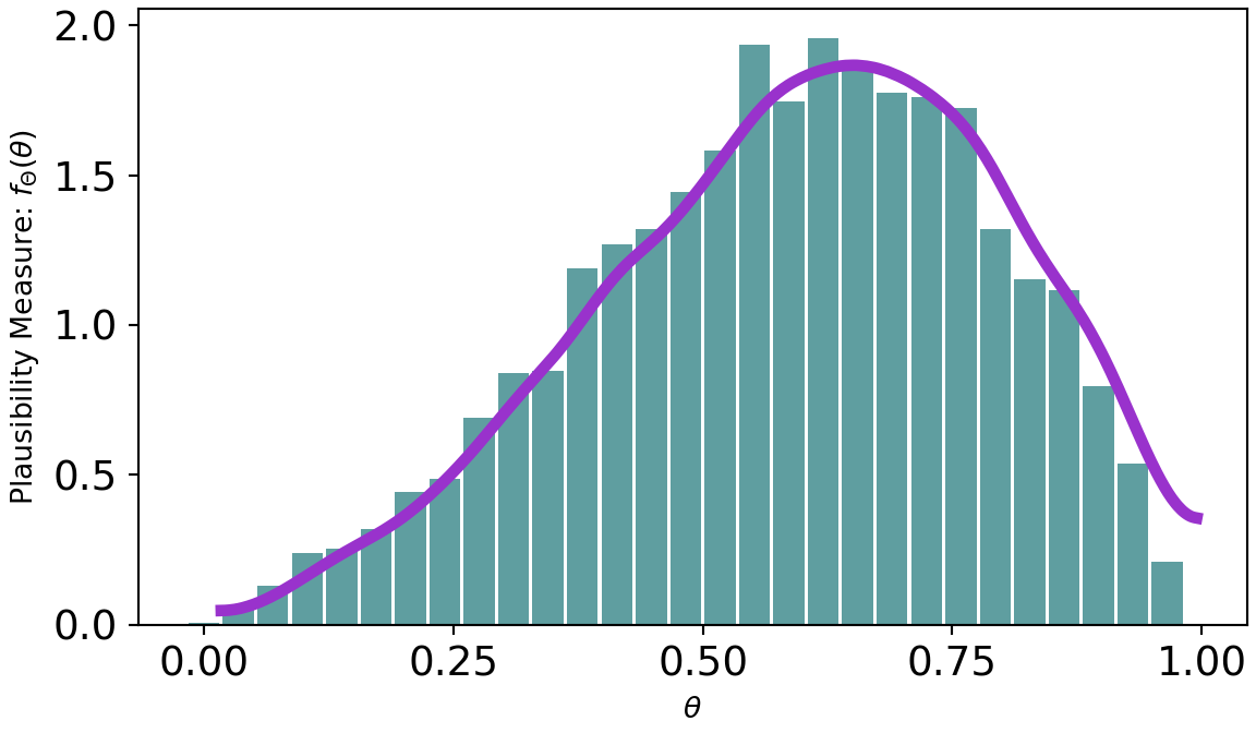
Figure 8.6: A prior beta(2,2) distribution along with the posterior distribution after observing 20 successes and two failures.

Figure 8.6 shows a dramatic shift from prior to posterior distribution. The weak prior suggest all values had plausibility, but once observing 20 successes out of 22 trials, the higher values for \(\theta\) are much more plausible.

If we want to change the prior to something stronger, say a \(\textrm{beta}(50,50)\), then we can rerun the numpyro code just changing the one line for the prior:

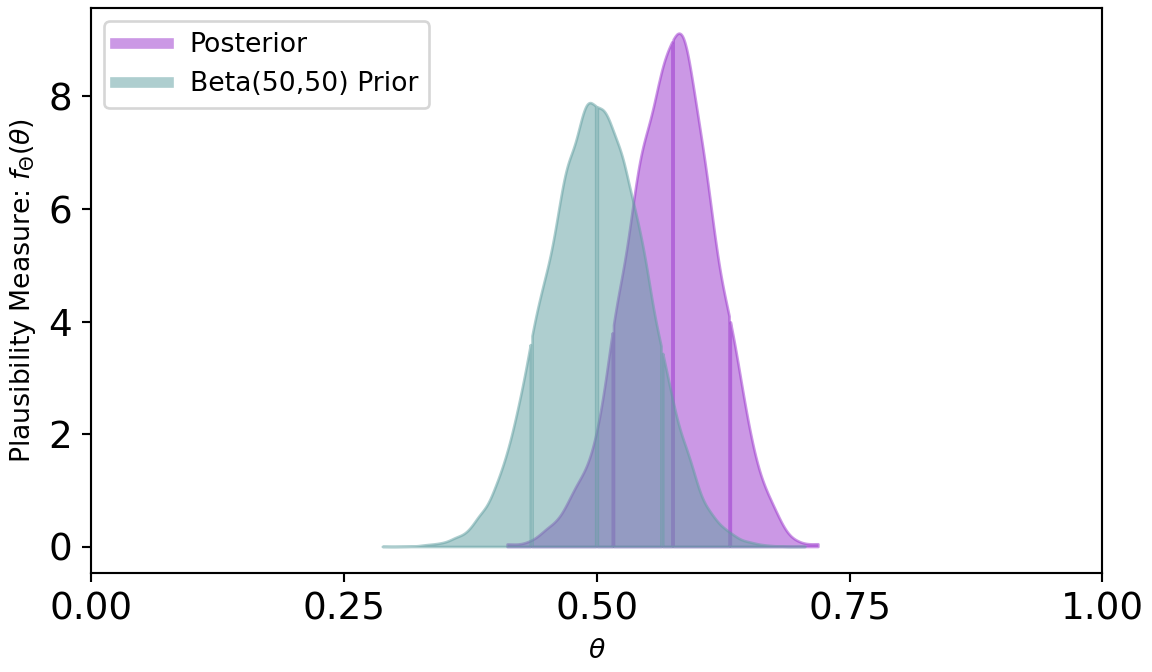
Figure 8.7: A prior beta(50,50) distribution along with the posterior distribution after observing 20 successes and two failures.

Figure 8.7 shows a posterior distribution that is only mildly shifted from its prior. This is a direct result of a strong prior due to the larger \(\alpha\) and \(\beta\) parameters. In general, we will not use strong priors and seek weakly informative priors that yield plausible prior generating processes, yet are flexible enough to let the data inform the posterior generating process. There is a bit of an art to this and we will learn more in subsequent chapters.

8.2 Getting Help

See the “Getting Started” section of the numpyro documentation for more details about coding in numpyro. A link to that section is here: https://num.pyro.ai/en/stable/getting_started.html.

8.3 Questions to Learn From

See CANVAS.